This page is part of the University of Colorado-Anschutz Medical Campus’ BIOS 6618 Labs collection, the mini-lecture content delivered at the start of class before breaking out into small groups to work on the homework assignment.
What’s on the docket this week?
We are diving into some examples of interactions and how to conduct inference on them (a notoriously tricky topic!). We’ll then spend the rest of time breaking out into groups to work on homework.
Interactions: Definition
Effect modification or interaction is when the relationship between our outcome, \(Y\), and primary explanatory variable (PEV), \(X\), varies by some other covariate, \(C\). Specifically the terms are defined as:
Effect Modification: non-quantitative clinical or biological attribute of population
Interaction: quantitative attribute of a dataset, may be scale dependent
An effect modifier or moderator is the variable that “causes” the effect modification. If a variable is an effect modifier, the role as a possible confounder is secondary.
Interactions Example from FEV Dataset
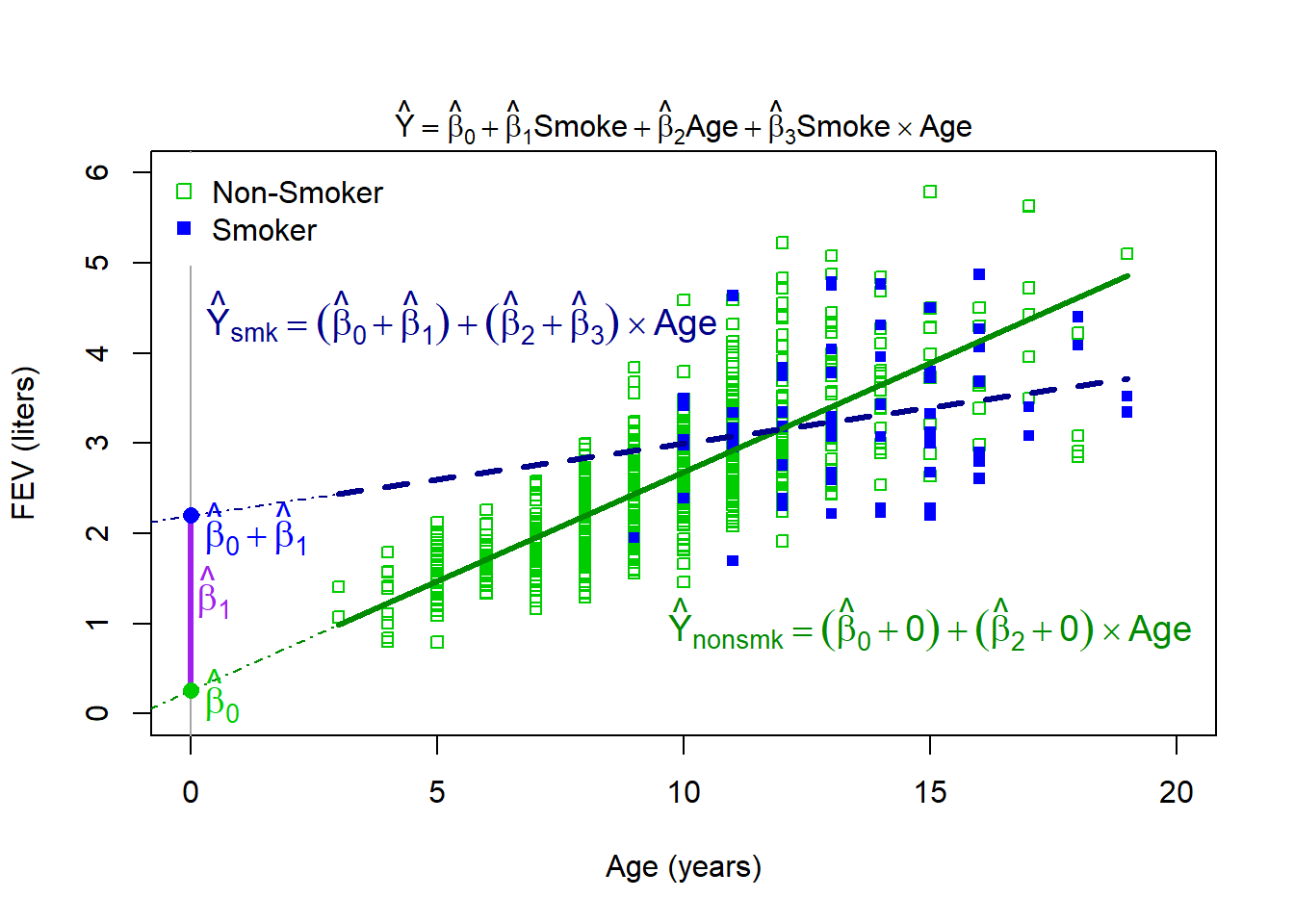
In our slide deck on effect modification we examined Rosner’s FEV dataset for the outcome of FEV predicted by smoking status (smoker vs. non-smoker), age (from 3 to 19), and their interaction. The fitted regression model was
The Regression Equation for Smokers vs. Non-smokers
Given that smoking status is a categorical predictor, we may be interested in using the fitted regression model above and simplifying it to be from the perspective of nonsmokers and smokers. This can help us more clearly identify the intercept and slope(s) for the two groups.
For non-smokers we can think of this as taking our fitted regression equation from above, plugging in “0” for “Smoker”, and focusing on simplified regression equation:
With these two regression equations, we can see that smokers and nonsmokers have different intercepts and slopes for age. We can also see that the intercept and slope for smokers is based on the sum of different \(\hat\beta\)’s. Visually this would look something like:
\(\hat\beta_0\): estimated average FEV for non-smokers at age 0 (i.e., all \(X=0\))
\(\hat\beta_1\): estimated difference in FEV at age 0 between smokers and non-smokers (i.e., difference in intercepts)
\(\hat\beta_2\): estimated slope for age for non-smokers (increase in FEV per year of age for non-smokers)
\(\hat\beta_3\): estimated difference in slope between smokers and non-smokers
\(\hat\beta_0 + \hat\beta_1\): estimated average FEV for smokers at age 0 (i.e., here \(X_1=1\), but \(X_1=0\) still)
\(\hat\beta_2 + \hat\beta_3\): estimated slope for age for smokers (increase in FEV per year of age for smokers)
Based on our interpretation above, we may be interested in formally testing the hypothesis that any one of our estimates is significantly different from 0. Fortunately, if we wish to test any of the \(\hat\beta\)’s on their own (i.e., not \(\hat\beta_i + \hat\beta_j\)), we can simply use the regression output:
                  Estimate Std. Error   t value      Pr(>|t|)
(Intercept)      0.2533955 0.08265075  3.065859  2.260474e-03
smokesmoker      1.9435707 0.41428463  4.691390  3.309624e-06
age              0.2425584 0.00833154 29.113274 6.504859e-120
smokesmoker:age -0.1627027 0.03073753 -5.293290  1.645078e-07
Inference for Non-Smokers (i.e., the Reference Category)
For example, for \(\hat\beta_2\) we would be testing if the estimated slope for age for non-smokers is significantly different from 0. We see that \(p<0.001\), so we would reject \(H_0\) and conclude that the slope for age for non-smokers is significantly different from 0.
The point estimate, interval estimate, and uncertainty for the association between FEV and age for non-smokers is:
Point Estimate: \(\hat{\beta}_2=\) 0.24256 liters/year
On average, FEV increases by 0.24 liters for a one year increase in age (95% CI: 0.23, 0.26 L) for non-smokers, which is significantly different from 0 (p<0.001).
Inference for Smokers
But if we are interested in testing the slope for age for smokers we need to do a little more work! There are 3 approaches that may be of use depending on the information you have available:
Calculate the standard error for \(\hat\beta_2 + \hat\beta_3\) by hand from the variance-covariance matrix to use in calculating 95% CI, p-values, etc.
Use some form of general linear hypothesis testing to do this work of combining beta coefficients.
Reverse code the categorical variable so that “Age” is now the estimated slope for age for smokers.
Option 1: Use the Variance-Covariance Matrix
Recall, the variance for two random variables that are added together is \(Var(X+Y) = Var(X) + Var(Y) + 2 \times Cov(X,Y)\). The standard error is then the square root of this: \(SE(X+Y) = \sqrt{Var(X+Y)}\).
We can replace \(X\) and \(Y\) with our \(\hat\beta\)’s of interest and calculate the standard error by extracting the relevant information from the variance-covariance matrix. The variance-covariance matrix is a square matrix (i.e., same number of rows and columns) which has the variances along the main diagonal (i.e., from upper left to lower right) and the covariances between any two beta coefficients on the off-diagonal:
Uncertainty: \(t=\frac{0.07986}{0.029587}=2.699\) with \(p=\)2*pt(2.699,650,lower.tail=F)\(=0.007\)
On average, FEV increases by 0.08 liters for a one year increase in age (95% CI: 0.02, 0.14 L) for smokers, which is significantly different from 0 (p=0.007).
Option 2: Use General Linear Hypothesis Tests
We can also use the glht function in the multcomp package in R to calculate the interval estimate and uncertainty:
                         Estimate Std. Error   t value     Pr(>|t|)
(Intercept)            2.19696626 0.40595641  5.411828 8.782811e-08
nonsmokenonsmoker     -1.94357074 0.41428463 -4.691390 3.309624e-06
age                    0.07985574 0.02958684  2.699029 7.134971e-03
nonsmokenonsmoker:age  0.16270267 0.03073753  5.293290 1.645078e-07
We see based on these results that the estimate, standard error, t-value, and p-value for age match our estimates from Options 1 and 2 above.
The caveat with this approach is that we would still have to fit the “original” model to estimate the effect for non-smokers without extra work, or we could do Option 1 or Option 2 for non-smokers with this model.
Source Code
---title: "Week 12 Lab"author: name: Alex Kaizer roles: "Instructor" affiliation: University of Colorado-Anschutz Medical Campustoc: truetoc_float: truetoc-location: leftformat: html: code-fold: show code-overflow: wrap code-tools: true---```{r, echo=F, message=F, warning=F}library(kableExtra)library(dplyr)```This page is part of the University of Colorado-Anschutz Medical Campus' [BIOS 6618 Labs](/labs/index.qmd) collection, the mini-lecture content delivered at the start of class before breaking out into small groups to work on the homework assignment.# What's on the docket this week?We are diving into some examples of interactions and how to conduct inference on them (a notoriously tricky topic!). We'll then spend the rest of time breaking out into groups to work on homework.# Interactions: DefinitionEffect modification or interaction is when the relationship between our outcome, $Y$, and primary explanatory variable (PEV), $X$, varies by some other covariate, $C$. Specifically the terms are defined as:* **Effect Modification:** non-quantitative clinical or biological attribute of *population** **Interaction:** quantitative attribute of a *dataset*, may be scale dependentAn **effect modifier** or **moderator** is the variable that "causes" the effect modification. If a variable is an effect modifier, the role as a possible confounder is secondary.# Interactions Example from FEV DatasetIn our slide deck on effect modification we examined Rosner's FEV dataset for the outcome of FEV predicted by smoking status (smoker vs. non-smoker), age (from 3 to 19), and their interaction. The fitted regression model was$\begin{aligned} \hat{Y} =& \hat\beta_0 + \hat\beta_1 X_1 + \hat\beta_2 X_2 + \hat\beta_3 X_1 X_2 \\=& 0.25 + 1.94 \times \text{Smoker} + 0.24 \times \text{Age} + (-0.16 \times \text{Smoker} \times \text{Age} ) \end{aligned}$## The Regression Equation for Smokers vs. Non-smokersGiven that smoking status is a categorical predictor, we may be interested in using the fitted regression model above and simplifying it to be from the perspective of nonsmokers and smokers. This can help us more clearly identify the intercept and slope(s) for the two groups.For *non-smokers* we can think of this as taking our fitted regression equation from above, plugging in "0" for "Smoker", and focusing on simplified regression equation:$\begin{aligned}\hat{Y}_{nonsmk} =& 0.25 + 1.94 \times 0 + 0.24 \times \text{Age} + (-0.16 \times 0 \times \text{Age} ) \\=& 0.25 + 0.24 \times \text{Age}\end{aligned}$Likewise, for *smokers* we can think of this as plugging in "1" for "Smoker":$\begin{aligned}\hat{Y}_{smk} =& 0.25 + 1.94 \times 1 + 0.24 \times \text{Age} + (-0.16 \times 1 \times \text{Age} ) \\=& (0.25+1.94) + (0.24-0.16) \times \text{Age} \\=& 2.19 + 0.08 \times \text{Age}\end{aligned}$With these two regression equations, we can see that smokers and nonsmokers have different intercepts and slopes for age. We can also see that the intercept and slope for *smokers* is based on the sum of different $\hat\beta$'s. Visually this would look something like:```{r, eval=T}#| code-fold: truefev <-read.csv('../../.data/FEV_rosner.csv')fev$pch <-0; fev$pch[which(fev$smoke=='smoker')] <-15fev$col <-'green3'; fev$col[which(fev$smoke=='smoker')] <-'blue'# Code to generate picture#FEV figure with regression lines for FEV ~ smoking status + age + smoke*age (slide 11)lmfi <-lm( fev ~ smoke * age, data=fev)plot(x=fev$age, y=fev$fev, pch=fev$pch,col=fev$col,cex=0.8, xlab='Age (years)', ylab='FEV (liters)', xlim=c(0,20), ylim=c(0,6))points(x=fev$age[which(fev$smoke=='smoker')], y=fev$fev[which(fev$smoke=='smoker')], pch=fev$pch[which(fev$smoke=='smoker')],col=fev$col[which(fev$smoke=='smoker')],cex=0.8)lines(x=c(3,19), y=( coef(lmfi)[1]+coef(lmfi)[3]*c(3,19) ), lwd=3, col='green4' )lines(x=c(3,19), y=( coef(lmfi)[1]+coef(lmfi)[2] +coef(lmfi)[3]*c(3,19) +coef(lmfi)[4]*c(3,19) ) , lty=2, lwd=3, col='blue4')lines(x=c(-1,3), y=( coef(lmfi)[1]+coef(lmfi)[3]*c(-1,3) ), lty=4, col='green4' )lines(x=c(-1,3), y=( coef(lmfi)[1]+coef(lmfi)[2] +coef(lmfi)[3]*c(-1,3)+coef(lmfi)[4]*c(-1,3) ) , lty=4, col='blue4')abline(v=0, col='gray65', lty=1)legend('topleft',inset=0.005,bg='white',box.col='white',pch=c(0,15),col=c('green3','blue'),legend=c('Non-Smoker','Smoker'))mtext( expression(hat(Y) ==hat(beta)[0] +hat(beta)[1] * Smoke +hat(beta)[2] * Age +hat(beta)[3] * Smoke %*% Age) )text(x =15, y =1, expression(hat(Y)[nonsmk] == (hat(beta)[0]+0) + (hat(beta)[2] +0) %*% Age), col='green4', cex=1.2)text(x =5.5, y =4.4, expression(hat(Y)[smk] == (hat(beta)[0]+hat(beta)[1]) + (hat(beta)[2] +hat(beta)[3]) %*% Age), col='blue4', cex=1.2)lines(x=c(0,0), y=c(coef(lmfi)[1],coef(lmfi)[1]+coef(lmfi)[2]), col='purple', lwd=3)text(x=-.25, y=1.3, expression(hat(beta)[1]), col='purple', pos=4, cex=1.2)text(x=-.1, y=0.15, expression(hat(beta)[0]), col='green3', pos=4, cex=1.2); points(x=0,y=coef(lmfi)[1], pch=16, col='green3', cex=1.2)text(x=-.1, y=2, expression(hat(beta)[0] +hat(beta)[1]), col='blue', pos=4, cex=1.2); points(x=0,y=coef(lmfi)[1]+coef(lmfi)[2], pch=16, col='blue', cex=1.2)```## Interpreting the Beta CoefficientsThe meaning of each $\hat{\beta}$ is:* $\hat\beta_0$: estimated average FEV for non-smokers at age 0 (i.e., all $X=0$)* $\hat\beta_1$: estimated difference in FEV at age 0 between smokers and non-smokers (i.e., difference in intercepts)* $\hat\beta_2$: estimated slope for age for *non-smokers* (increase in FEV per year of age for non-smokers)* $\hat\beta_3$: estimated *difference* in slope between smokers and non-smokers* $\hat\beta_0 + \hat\beta_1$: estimated average FEV for smokers at age 0 (i.e., here $X_1=1$, but $X_1=0$ still)* $\hat\beta_2 + \hat\beta_3$: estimated slope for age for *smokers* (increase in FEV per year of age for smokers)Based on our interpretation above, we may be interested in formally testing the hypothesis that any one of our estimates is significantly different from 0. Fortunately, if we wish to test any of the $\hat\beta$'s on their own (i.e., not $\hat\beta_i + \hat\beta_j$), we can simply use the regression output:```{r, class.source='fold-show'}mod1 <-lm( fev ~ smoke * age, data=fev)summary(mod1)$coefficients```## Inference for Non-Smokers (i.e., the Reference Category)For example, for $\hat\beta_2$ we would be testing if the estimated slope for age for *non-smokers* is significantly different from 0. We see that $p<0.001$, so we would reject $H_0$ and conclude that the slope for age for non-smokers is significantly different from 0.The point estimate, interval estimate, and uncertainty for the association between FEV and age for *non-smokers* is:* Point Estimate: $\hat{\beta}_2=$ 0.24256 liters/year* Interval Estimate (95% CI): $\hat{\beta}_2 \pm t_{n-p-1,\alpha/2} SE(\hat{\beta}_2) = 0.24256 \pm 1.96(0.00833) = (0.2262, 0.2589)$, where $t_{650,0.975}=1.96$* Uncertainty: $t=29.11$ with $p<0.001$On average, FEV increases by 0.24 liters for a one year increase in age (95% CI: 0.23, 0.26 L) for non-smokers, which is significantly different from 0 (p<0.001).## Inference for Smokers**But if we are interested in testing the slope for age for smokers we need to do a little more work!** There are 3 approaches that may be of use depending on the information you have available:1. Calculate the standard error for $\hat\beta_2 + \hat\beta_3$ by hand from the variance-covariance matrix to use in calculating 95% CI, p-values, etc.2. Use some form of general linear hypothesis testing to do this work of combining beta coefficients.3. Reverse code the categorical variable so that "Age" is now the estimated slope for age for *smokers*.## Option 1: Use the Variance-Covariance MatrixRecall, the variance for two random variables that are added together is $Var(X+Y) = Var(X) + Var(Y) + 2 \times Cov(X,Y)$. The standard error is then the square root of this: $SE(X+Y) = \sqrt{Var(X+Y)}$.We can replace $X$ and $Y$ with our $\hat\beta$'s of interest and calculate the standard error by extracting the relevant information from the variance-covariance matrix. The *variance-covariance* matrix is a square matrix (i.e., same number of rows and columns) which has the variances along the main diagonal (i.e., from upper left to lower right) and the covariances between any two beta coefficients on the off-diagonal:```{r, class.source='fold-show'}vcov(mod1)```From this matrix we see that * $Var(\hat\beta_2)=6.941456e-05=0.0000694146$* $Var(\hat\beta_3)=9.447957e-04=0.0009447957$* $Cov(\hat\beta_2,\hat\beta_3)=Cov(\hat\beta_3,\hat\beta_2)=-6.941456e-05=−0.000069415$Plugging these values into our equation for the standard error results in:$\begin{aligned}SE(\hat{\beta}_2+\hat{\beta}_3) =& \sqrt{Var(\hat{\beta}_2) + Var(\hat{\beta}_3) + 2\times Cov(\hat{\beta}_2,\hat{\beta}_3)} \\=& \sqrt{0.0000694146 + 0.0009447957 + 2(-0.000069415)} \\=& \sqrt{0.0008753803} \\=& 0.029587\end{aligned}$The point estimate, interval estimate, and uncertainty for the association between FEV and age for *smokers* is:* Point Estimate: $\hat{\beta}_2 + \hat{\beta}_3=0.24256+(-0.16270)=$ 0.07986 liters/year* Interval Estimate (95% CI): $0.07986 \pm 1.96(0.029587) = (0.0219, 0.1378)$* Uncertainty: $t=\frac{0.07986}{0.029587}=2.699$ with $p=$`2*pt(2.699,650,lower.tail=F)`$=0.007$On average, FEV increases by 0.08 liters for a one year increase in age (95% CI: 0.02, 0.14 L) for smokers, which is significantly different from 0 (p=0.007).## Option 2: Use General Linear Hypothesis TestsWe can also use the `glht` function in the `multcomp` package in `R` to calculate the interval estimate and uncertainty:```{r,echo=T, message=F, class.source='fold-show'}library(multcomp)K <-matrix(c(0,0,1,1),nrow=1) #beta2+beta3summary(glht(mod1, linfct=K))```We see that the results match those of Option 1.**NOTE:** For `glm` models the normal approximation is used, whereas for `lm` models the t-distribution is used.## Option 3: Use Reverse Coding of the Categorical PredictorOur third option is to reverse the coding for `smoke`, then evaluate the estimate of the new $\hat\beta_2^*$:```{r, class.source='fold-show'}fev$nonsmoke <-factor(fev$smoke, levels=c('smoker','nonsmoker'))mod1_reverse <-lm( fev ~ nonsmoke*age, data=fev )summary(mod1_reverse)$coefficients```We see based on these results that the estimate, standard error, t-value, and p-value for `age` match our estimates from Options 1 and 2 above.The caveat with this approach is that we would still have to fit the "original" model to estimate the effect for non-smokers without extra work, *or* we could do Option 1 or Option 2 for non-smokers with this model.