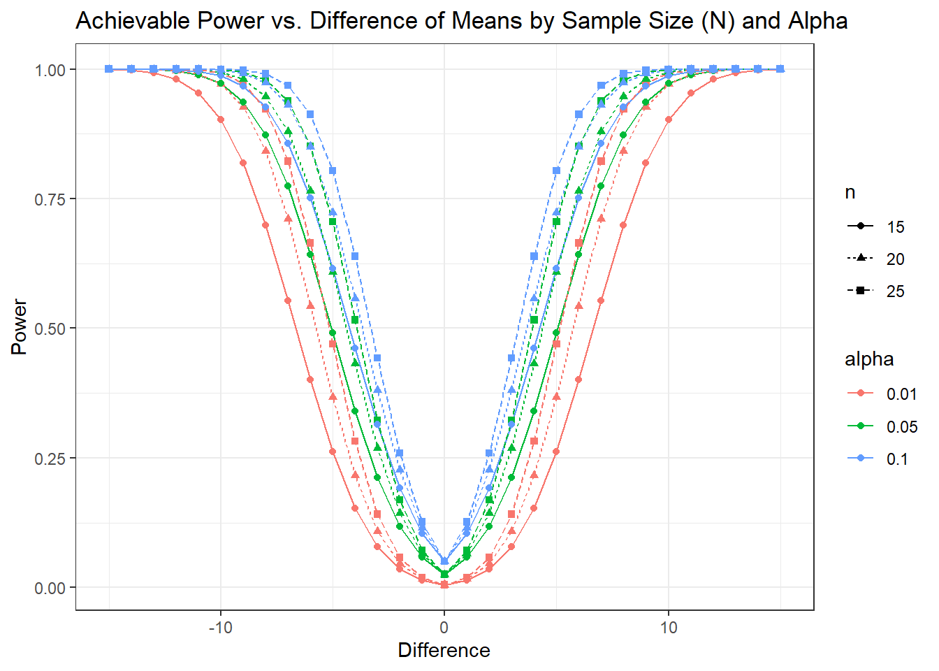
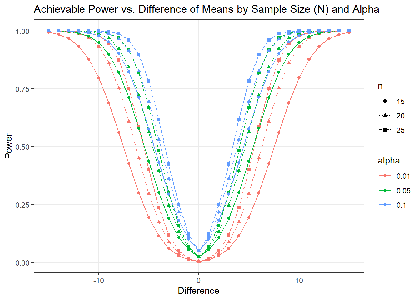
     One-sample t test power calculation

              n = 15, 20, 25, 15, 20, 25, 15, 20, 25, 15, 20, 25, 15, 20, 25, 15, 20, 25, 15, 20, 25, 15, 20, 25, 15, 20, 25, 15, 20, 25, 15, 20, 25, 15, 20, 25, 15, 20, 25, 15, 20, 25, 15, 20, 25, 15, 20, 25, 15, 20, 25, 15, 20, 25, 15, 20, 25, 15, 20, 25, 15, 20, 25, 15, 20, 25, 15, 20, 25, 15, 20, 25, 15, 20, 25, 15, 20, 25, 15, 20, 25, 15, 20, 25, 15, 20, 25, 15, 20, 25, 15, 20, 25, 15, 20, 25, 15, 20, 25, 15, 20, 25, 15, 20, 25, 15, 20, 25, 15, 20, 25, 15, 20, 25, 15, 20, 25, 15, 20, 25, 15, 20, 25, 15, 20, 25, 15, 20, 25, 15, 20, 25, 15, 20, 25, 15, 20, 25, 15, 20, 25, 15, 20, 25, 15, 20, 25, 15, 20, 25, 15, 20, 25, 15, 20, 25, 15, 20, 25, 15, 20, 25, 15, 20, 25, 15, 20, 25, 15, 20, 25, 15, 20, 25, 15, 20, 25, 15, 20, 25, 15, 20, 25, 15, 20, 25, 15, 20, 25, 15, 20, 25, 15, 20, 25, 15, 20, 25, 15, 20, 25, 15, 20, 25, 15, 20, 25, 15, 20, 25, 15, 20, 25, 15, 20, 25, 15, 20, 25, 15, 20, 25, 15, 20, 25, 15, 20, 25, 15, 20, 25, 15, 20, 25, 15, 20, 25, 15, 20, 25, 15, 20, 25, 15, 20, 25, 15, 20, 25, 15, 20, 25, 15, 20, 25, 15, 20, 25, 15, 20, 25, 15, 20, 25, 15, 20, 25, 15, 20, 25, 15, 20, 25, 15, 20, 25, 15, 20, 25
          delta = 15, 15, 15, 15, 15, 15, 15, 15, 15, 14, 14, 14, 14, 14, 14, 14, 14, 14, 13, 13, 13, 13, 13, 13, 13, 13, 13, 12, 12, 12, 12, 12, 12, 12, 12, 12, 11, 11, 11, 11, 11, 11, 11, 11, 11, 10, 10, 10, 10, 10, 10, 10, 10, 10, 9, 9, 9, 9, 9, 9, 9, 9, 9, 8, 8, 8, 8, 8, 8, 8, 8, 8, 7, 7, 7, 7, 7, 7, 7, 7, 7, 6, 6, 6, 6, 6, 6, 6, 6, 6, 5, 5, 5, 5, 5, 5, 5, 5, 5, 4, 4, 4, 4, 4, 4, 4, 4, 4, 3, 3, 3, 3, 3, 3, 3, 3, 3, 2, 2, 2, 2, 2, 2, 2, 2, 2, 1, 1, 1, 1, 1, 1, 1, 1, 1, 0, 0, 0, 0, 0, 0, 0, 0, 0, 1, 1, 1, 1, 1, 1, 1, 1, 1, 2, 2, 2, 2, 2, 2, 2, 2, 2, 3, 3, 3, 3, 3, 3, 3, 3, 3, 4, 4, 4, 4, 4, 4, 4, 4, 4, 5, 5, 5, 5, 5, 5, 5, 5, 5, 6, 6, 6, 6, 6, 6, 6, 6, 6, 7, 7, 7, 7, 7, 7, 7, 7, 7, 8, 8, 8, 8, 8, 8, 8, 8, 8, 9, 9, 9, 9, 9, 9, 9, 9, 9, 10, 10, 10, 10, 10, 10, 10, 10, 10, 11, 11, 11, 11, 11, 11, 11, 11, 11, 12, 12, 12, 12, 12, 12, 12, 12, 12, 13, 13, 13, 13, 13, 13, 13, 13, 13, 14, 14, 14, 14, 14, 14, 14, 14, 14, 15, 15, 15, 15, 15, 15, 15, 15, 15
             sd = 10
      sig.level = 0.01, 0.01, 0.01, 0.05, 0.05, 0.05, 0.10, 0.10, 0.10, 0.01, 0.01, 0.01, 0.05, 0.05, 0.05, 0.10, 0.10, 0.10, 0.01, 0.01, 0.01, 0.05, 0.05, 0.05, 0.10, 0.10, 0.10, 0.01, 0.01, 0.01, 0.05, 0.05, 0.05, 0.10, 0.10, 0.10, 0.01, 0.01, 0.01, 0.05, 0.05, 0.05, 0.10, 0.10, 0.10, 0.01, 0.01, 0.01, 0.05, 0.05, 0.05, 0.10, 0.10, 0.10, 0.01, 0.01, 0.01, 0.05, 0.05, 0.05, 0.10, 0.10, 0.10, 0.01, 0.01, 0.01, 0.05, 0.05, 0.05, 0.10, 0.10, 0.10, 0.01, 0.01, 0.01, 0.05, 0.05, 0.05, 0.10, 0.10, 0.10, 0.01, 0.01, 0.01, 0.05, 0.05, 0.05, 0.10, 0.10, 0.10, 0.01, 0.01, 0.01, 0.05, 0.05, 0.05, 0.10, 0.10, 0.10, 0.01, 0.01, 0.01, 0.05, 0.05, 0.05, 0.10, 0.10, 0.10, 0.01, 0.01, 0.01, 0.05, 0.05, 0.05, 0.10, 0.10, 0.10, 0.01, 0.01, 0.01, 0.05, 0.05, 0.05, 0.10, 0.10, 0.10, 0.01, 0.01, 0.01, 0.05, 0.05, 0.05, 0.10, 0.10, 0.10, 0.01, 0.01, 0.01, 0.05, 0.05, 0.05, 0.10, 0.10, 0.10, 0.01, 0.01, 0.01, 0.05, 0.05, 0.05, 0.10, 0.10, 0.10, 0.01, 0.01, 0.01, 0.05, 0.05, 0.05, 0.10, 0.10, 0.10, 0.01, 0.01, 0.01, 0.05, 0.05, 0.05, 0.10, 0.10, 0.10, 0.01, 0.01, 0.01, 0.05, 0.05, 0.05, 0.10, 0.10, 0.10, 0.01, 0.01, 0.01, 0.05, 0.05, 0.05, 0.10, 0.10, 0.10, 0.01, 0.01, 0.01, 0.05, 0.05, 0.05, 0.10, 0.10, 0.10, 0.01, 0.01, 0.01, 0.05, 0.05, 0.05, 0.10, 0.10, 0.10, 0.01, 0.01, 0.01, 0.05, 0.05, 0.05, 0.10, 0.10, 0.10, 0.01, 0.01, 0.01, 0.05, 0.05, 0.05, 0.10, 0.10, 0.10, 0.01, 0.01, 0.01, 0.05, 0.05, 0.05, 0.10, 0.10, 0.10, 0.01, 0.01, 0.01, 0.05, 0.05, 0.05, 0.10, 0.10, 0.10, 0.01, 0.01, 0.01, 0.05, 0.05, 0.05, 0.10, 0.10, 0.10, 0.01, 0.01, 0.01, 0.05, 0.05, 0.05, 0.10, 0.10, 0.10, 0.01, 0.01, 0.01, 0.05, 0.05, 0.05, 0.10, 0.10, 0.10, 0.01, 0.01, 0.01, 0.05, 0.05, 0.05, 0.10, 0.10, 0.10
          power = 0.99379964, 0.99977175, 0.99999374, 0.99968449, 0.99999414, 0.99999991, 0.99994334, 0.99999923, 0.99999999, 0.98492058, 0.99904610, 0.99995370, 0.99890204, 0.99996285, 0.99999894, 0.99976298, 0.99999400, 0.99999987, 0.96672386, 0.99656180, 0.99971913, 0.99659928, 0.99980079, 0.99998997, 0.99912482, 0.99996071, 0.99999843, 0.93326751, 0.98929560, 0.99860140, 0.99061448, 0.99909540, 0.99992373, 0.99714477, 0.99978391, 0.99998523, 0.87812317, 0.97115118, 0.99427099, 0.97688373, 0.99651570, 0.99953252, 0.99175854, 0.99900034, 0.99988907, 0.79670393, 0.93249537, 0.98063807, 0.94908647, 0.98859129, 0.99768460, 0.97891618, 0.99610286, 0.99933233, 0.68910390, 0.86228289, 0.94578357, 0.89945099, 0.96815164, 0.99070503, 0.95208492, 0.98716538, 0.99677194, 0.56192862, 0.75363390, 0.87346165, 0.82130998, 0.92389872, 0.96963105, 0.90297615, 0.96417280, 0.98741901, 0.42761072, 0.61050606, 0.75174714, 0.71289906, 0.84350550, 0.91877622, 0.82425706, 0.91484955, 0.96028374, 0.30095252, 0.45011623, 0.58571735, 0.58040966, 0.72100197, 0.82072129, 0.71377695, 0.82663952, 0.89776394, 0.19441072, 0.29734431, 0.40227469, 0.43784659, 0.56448290, 0.66970136, 0.57805549, 0.69514934, 0.78338612, 0.11453654, 0.17375617, 0.23822547, 0.30284108, 0.39686955, 0.48396689, 0.43215762, 0.53181412, 0.61725900, 0.06121551, 0.08891184, 0.11957051, 0.19037733, 0.24648577, 0.30161925, 0.29495606, 0.36277965, 0.42572891, 0.02954918, 0.03952378, 0.05021130, 0.10800411, 0.13348840, 0.15876192, 0.18211929, 0.21707518, 0.25048467, 0.01283438, 0.01516757, 0.01747061, 0.05498090, 0.06241123, 0.06948589, 0.10098691, 0.11249211, 0.12326268, 0.00500000, 0.00500000, 0.00500000, 0.02500000, 0.02500000, 0.02500000, 0.05000000, 0.05000000, 0.05000000, 0.01283438, 0.01516757, 0.01747061, 0.05498090, 0.06241123, 0.06948589, 0.10098691, 0.11249211, 0.12326268, 0.02954918, 0.03952378, 0.05021130, 0.10800411, 0.13348840, 0.15876192, 0.18211929, 0.21707518, 0.25048467, 0.06121551, 0.08891184, 0.11957051, 0.19037733, 0.24648577, 0.30161925, 0.29495606, 0.36277965, 0.42572891, 0.11453654, 0.17375617, 0.23822547, 0.30284108, 0.39686955, 0.48396689, 0.43215762, 0.53181412, 0.61725900, 0.19441072, 0.29734431, 0.40227469, 0.43784659, 0.56448290, 0.66970136, 0.57805549, 0.69514934, 0.78338612, 0.30095252, 0.45011623, 0.58571735, 0.58040966, 0.72100197, 0.82072129, 0.71377695, 0.82663952, 0.89776394, 0.42761072, 0.61050606, 0.75174714, 0.71289906, 0.84350550, 0.91877622, 0.82425706, 0.91484955, 0.96028374, 0.56192862, 0.75363390, 0.87346165, 0.82130998, 0.92389872, 0.96963105, 0.90297615, 0.96417280, 0.98741901, 0.68910390, 0.86228289, 0.94578357, 0.89945099, 0.96815164, 0.99070503, 0.95208492, 0.98716538, 0.99677194, 0.79670393, 0.93249537, 0.98063807, 0.94908647, 0.98859129, 0.99768460, 0.97891618, 0.99610286, 0.99933233, 0.87812317, 0.97115118, 0.99427099, 0.97688373, 0.99651570, 0.99953252, 0.99175854, 0.99900034, 0.99988907, 0.93326751, 0.98929560, 0.99860140, 0.99061448, 0.99909540, 0.99992373, 0.99714477, 0.99978391, 0.99998523, 0.96672386, 0.99656180, 0.99971913, 0.99659928, 0.99980079, 0.99998997, 0.99912482, 0.99996071, 0.99999843, 0.98492058, 0.99904610, 0.99995370, 0.99890204, 0.99996285, 0.99999894, 0.99976298, 0.99999400, 0.99999987, 0.99379964, 0.99977175, 0.99999374, 0.99968449, 0.99999414, 0.99999991, 0.99994334, 0.99999923, 0.99999999
    alternative = two.sided