Code
if( condition ){
  run code if condition met
}This page is part of the University of Colorado-Anschutz Medical Campus’ BIOS 6618 Labs collection, the mini-lecture content delivered at the start of class before breaking out into small groups to work on the homework assignment.
In Week 5 we are introducing if statements, including if/else statements. These allow you to tell R to complete a certain step if and only if some criteria is met. We will also see different ways we can subset data. Finally, we have an example of a simulation study to evaluate the challenge of multiple testing in statistics.
if and else statements are great to employ certain conditions when you want to them complete a certain step. Sections 9.2-9.3 of our R Textbook discuss if and else statements and can serve as an additional reference.
ifThe if statement has a very simple structure:
if( condition ){
run code if condition met
}The condition must be something that is either TRUE or FALSE. If the condition is met, then R will run whatever code is contained between our curly brackets.
As an example, let’s write three if statements that generate a sample from either a normal or exponential distribution based on an object we defined called dist as either normal or exponential:
set.seed(561326)
dist <- 'exponential' # set desired distribution to simulate from

if(dist == 'exponential'){ rexp(n=10, rate=0.5) }
if(dist == 'normal'){ rnorm(n=10, mean=10, sd=4) }
[1] 0.46504343 2.52015675 4.16642691 1.00602212 0.63401942 0.01873791
[7] 2.80259386 1.18373900 5.37115794 4.67971633We could also make it more informative by also printing a character string that reminds us what distribution we selected:
set.seed(561326)
dist <- 'exponential' # set desired distribution to simulate from
if(dist == 'exponential'){
print('You requested the exponential distribution.')
rexp(n=10, rate=0.5)
}
if(dist == 'normal'){
print('You requested the normal distribution.')
rnorm(n=10, mean=10, sd=4)
}[1] "You requested the exponential distribution."
 [1] 0.46504343 2.52015675 4.16642691 1.00602212 0.63401942 0.01873791
[7] 2.80259386 1.18373900 5.37115794 4.67971633While this example includes two if statements, we could add as many as desired to complete a given task.
elseThe if statement will only run a set of code if the condition is TRUE, however we often will want to implement another set of code if the condition is FALSE. This is where the else statement comes in handy:
if( condition ){
  run code if condition met
}else{
  run this code instead if condition is NOT met
}
It is also possible to add additional if statements:
if( condition ){
  run code if condition met
}else if( condition2 ){
  run this code instead if condition IS NOT met but condition2 IS met
}else{
  run this code only if condition and condition2 are both NOT met
}
For example, perhaps we wish to simulate 100 standard normal data sets of \(n=10\) and want to count the number of times the mean is less than -0.5, between -0.5 and 0.5, and greater than 0.5. While there are multiple ways we could achieve this, let’s practice with if and else to achieve this:
set.seed(98512) # set seed for reproducibility

nsim <- 100
cat_vec <- rep(NA, length=nsim) # initialize object to store results in

for( i in 1:nsim ){
  asd <- rnorm(n=10)

  if( mean(asd) < -0.5){
    cat_vec[i] <- 'mean < -0.5'
  }else if(mean(asd) > 0.5){
    cat_vec[i] <- 'mean > 0.5'
  }else{
    cat_vec[i] <- 'mean between -0.5 and 0.5'
  }
}

table(cat_vec) #create a table summarizing results
cat_vec
mean < -0.5 mean > 0.5 mean between -0.5 and 0.5
6 6 88 There are a handful of different ways we have seen to subset or select specific aspects of a given object.
For example, we have seen using the index for both vectors and matrices. Let’s create a vector of length 5 and a 5x5 (row x column) matrix to illustrate this, where the elements are the location of the vector or row/column of the matrix from 1 to 5:
vec1 <- 1:5 # create a vector of length 5
vec1 # view the vector
[1] 1 2 3 4 5mat1 <- matrix( as.numeric(paste0( 1:5, matrix( rep(1:5,each=5), nrow=5))), nrow=5) #create a matrix with each coordinate being its combination of row and column
mat1 # print the matrix [,1] [,2] [,3] [,4] [,5]
[1,] 11 12 13 14 15
[2,] 21 22 23 24 25
[3,] 31 32 33 34 35
[4,] 41 42 43 44 45
[5,] 51 52 53 54 55For example, if we wanted to see the 4th element of our vector:
vec1[4][1] 4We see that it is the expected value 4.
If we wanted to see the 4th column of our matrix:
mat1[,4] # select entire fourth column[1] 14 24 34 44 54We see we have the values 14, 24, 34, 44, and 54 to reflect the 5 different rows and our column.
Likewise, we can do the same for the entire 4th row of the our matrix:
mat1[4,][1] 41 42 43 44 45Additionally, we can select a single element of the matrix by providing both a row and column coordinate. For example, we can call the 2nd row and 4th column:
mat1[2,4][1] 24Here we see the value is 24, as expected for the requested location.
Data frames always have column names (but can also be selected by index). Unique row names are optional for data frames (that aren’t just the number of the row). For vectors and matrices names are also optional, but can be helpful.
When we do have a name, we can specifically request the data by name. Let’s create a small data frame of the dogs in the Kaizer family to see this behavior:
my_df <- data.frame(
  dog_name=c('Baisy','Kaizer','Yahtzee','Sheba'),
  state=c('CO','IA','IA','VA'),
  size=c('med','large','small','med'),
  est_age=c(7,10,2,11)
)

my_df # print data frame
dog_name state size est_age
1 Baisy CO med 7
2 Kaizer IA large 10
3 Yahtzee IA small 2
4 Sheba VA med 11We the data frame contains information in both numeric and character formats. If we wanted to extract the column of dog names we could request the data in three different ways:
my_df[,1] # by column number[1] "Baisy" "Kaizer" "Yahtzee" "Sheba" my_df[,'dog_name'] # by column name in the [row,column] structure similar to a matrix[1] "Baisy" "Kaizer" "Yahtzee" "Sheba" my_df$dog_name # by column name using only the "$" operator[1] "Baisy" "Kaizer" "Yahtzee" "Sheba" We can see that all 3 approaches correctly pull the column containing the names of the puppers.
One way we may wish to subset data is by applying a logical rule, where values with TRUE are retained and FALSE removed. For example, let’s say we wish to subset by dogs living in Iowa:
my_df[ my_df$state=='IA', ] # extract the dogs who live in Iowa dog_name state size est_age
2 Kaizer IA large 10
3 Yahtzee IA small 2We see that Kaizer and Yahtzee were correctly subset.
Another similar approach is to use the which() function, which returns the indices where the statement is true:
which( my_df$state == 'IA' ) # check which indices match this value[1] 2 3my_df[ which( my_df$state == 'IA' ), ] # extract the dogs who live in Iowa dog_name state size est_age
2 Kaizer IA large 10
3 Yahtzee IA small 2The use of which() resulted in the same subset that was desired.
We can also subset based on conditions involving our numeric variable estimated age:
my_df[ which( my_df$est_age <= 8),] # subset to dogs less than or equal to 8 years of age dog_name state size est_age
1 Baisy CO med 7
3 Yahtzee IA small 2I generally prefer using which() because I have occasionally run into issues without it.
Another consideration is that we can match multiple elements in a column or have multiple conditions. For multiple elements instead of == we can use %in%. An example of subsetting based on a dog living in Iowa or Virginia is
my_df[ which( my_df$state %in% c('IA','VA') ),] # subset dogs living in Iowa or Virginia dog_name state size est_age
2 Kaizer IA large 10
3 Yahtzee IA small 2
4 Sheba VA med 11If we accidentally used == we see an incorrect subset:
my_df[ which( my_df$state == c('IA','VA') ),] # note the incorrect subset when using == dog_name state size est_age
3 Yahtzee IA small 2
4 Sheba VA med 11Where did Kaizer go?! It turns out the R repeated the c('IA','VA') vector so it was really matching c('IA','VA','IA','VA') to our vector of c('CO','IA','IA','VA').
For multiple conditions we can either use & (and) to indicate both conditions are met or | (or) to indicate either condition is met. An example of matching Iowa and small dogs is:
my_df[ which( my_df$state=='IA' & my_df$size=='small' ),] # subset rows where both conditions are TRUE dog_name state size est_age
3 Yahtzee IA small 2An example of matching Colorado or medium size is:
my_df[ which( my_df$state=='CO' | my_df$size=='med'),] dog_name state size est_age
1 Baisy CO med 7
4 Sheba VA med 11Multiple testing or multiple comparison issues arise in many cases when you conduct more than one statistical test. In some contexts the issue is built into the methodology (e.g., an ANOVA followed by a post-hoc test), but in other cases it is the result of a study design (e.g., having multiple outcomes of interest). We’ll approach the situation more generally where we have a study with 10 different hypothesis tests being conducted.
One of the easiest ways to see the impact of our choices on multiple testing correction is to conduct a simulation study. We’ll focus on the two extremes, one where all 10 hypothesis tests are null and one where all 10 hypothesis tests are an alternative. And to focus on the trade-off of both marginal and family-wise type I error rates with power, we’ll summarize the performance of all 3.
As our motivating context, we wish to design a clinical trial where we want to detect a mean difference of 10 mg/dL in total cholesterol over the course of an intervention in a study comparing two groups. We have preliminary data that suggests the expected standard deviation is 15 mg/dL. Our sample size, assuming \(\alpha=0.05\) and 80% power, is
power.t.test(delta=10, sd=15, sig.level=0.05, power=0.8)
     Two-sample t test power calculation

              n = 36.3058
          delta = 10
             sd = 15
      sig.level = 0.05
          power = 0.8
    alternative = two.sided

NOTE: n is number in *each* group
Based on our power.t.test calculation, we would need to enroll 37 participants per group. With this information in mind, let’s explore some simulation studies with 1000 simulated trials with 10 hypotheses.
First we’ll start with the null scenario, where each group will have a simulated mean change of 0 over the course of the study. For each study we will save the uncorrected p-value, the Bonferroni corrected p-value, and the false discovery rate (FDR) corrected p-value. From our simulation study we will then be able to calculate:
# Step 1: set the seed for reproducibility
set.seed(1117)

# Step 2: define variables of interest (that will be easy to change for different simulations)
nsim <- 1000 # number of simulations
nhyp <- 10 # number of hypothesis tests
alpha <- 0.05 # type I error rate

# set simulation parameters for data:
mean_grp1 <- 0
mean_grp2 <- 0
sd_grp1 <- 15
sd_grp2 <- 15
n_grp1 <- 37
n_grp2 <- 37

# Step 3: initialize a matrix to store our results in for each test based on our 3 approaches
null_mat <- matrix(nrow=nsim, ncol=nhyp*3)
colnames( null_mat ) <- c( paste0('original_p_',1:nhyp), paste0('fdr_p_',1:nhyp), paste0('bonf_p_',1:nhyp) )

# Step 4: simulate the trials and hypotheses, store the p-value results
for(i in 1:nsim){
  simdat_grp1 <- matrix( rnorm( n=n_grp1*nhyp, mean=mean_grp1, sd=sd_grp1 ), ncol=nhyp, nrow=n_grp1, byrow=FALSE)
  simdat_grp2 <- matrix( rnorm( n=n_grp2*nhyp, mean=mean_grp2, sd=sd_grp2 ), ncol=nhyp, nrow=n_grp2, byrow=FALSE)

  pvec_orig <- sapply( 1:nhyp, function(x) t.test(x=simdat_grp1[,x], y=simdat_grp2[,x])$p.value )
  pvec_fdr <- p.adjust( pvec_orig, method='fdr')
  pvec_bonf <- p.adjust( pvec_orig, method='bonferroni')

  null_mat[i,] <- c(pvec_orig, pvec_fdr, pvec_bonf)
}
Before summarizing the type I error rates, let’s first examine some histograms of our overall collection of p-values from the 10 tests:
par(mfrow=c(1,3))
hist(null_mat[,paste0('original_p_',1:nhyp)], main='Uncorrected p-value', xlab='p-value', ylim=c(0,10000))
hist(null_mat[,paste0('fdr_p_',1:nhyp)], main='FDR Corrected p-value', xlab='p-value', ylim=c(0,10000))
hist(null_mat[,paste0('bonf_p_',1:nhyp)], main='Bonferroni Corrected p-Value', xlab='p-value', ylim=c(0,10000))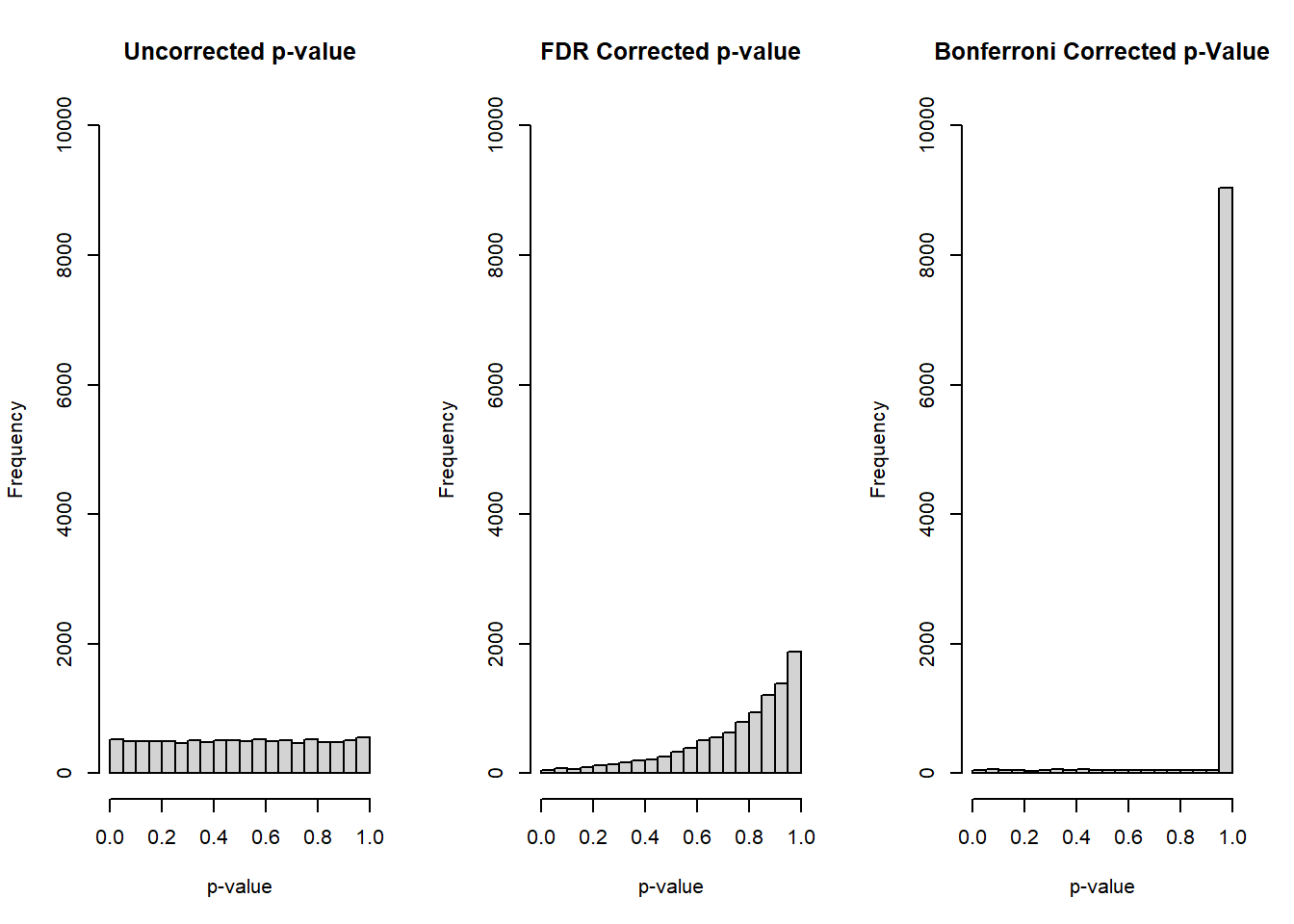
The uncorrected p-value from our \(10 \times 1000 = 10000\) total tests reflects the expected behavior for a null response, a uniform distribution. For both corrections, FDR and Bonferroni, we see that the distribution is skewed towards higher p-values, representing that post-hoc correction being applied to our tests.
Now let’s summarize our marginal and family-wise type I error rates:
library(kableExtra)

orig_marg_t1e <- mean( null_mat[,paste0('original_p_',1:nhyp)] <= alpha )
fdr_marg_t1e <- mean( null_mat[,paste0('fdr_p_',1:nhyp)] <= alpha )
bonf_marg_t1e <- mean( null_mat[,paste0('bonf_p_',1:nhyp)] <= alpha )

orig_fw_t1e <- mean( rowSums(null_mat[,paste0('original_p_',1:nhyp)] <= alpha) > 0 )
fdr_fw_t1e <- mean( rowSums(null_mat[,paste0('fdr_p_',1:nhyp)] <= alpha) > 0  )
bonf_fw_t1e <- mean( rowSums(null_mat[,paste0('bonf_p_',1:nhyp)] <= alpha) > 0  )

res_tab <- matrix( c(orig_marg_t1e,fdr_marg_t1e,bonf_marg_t1e, orig_fw_t1e, fdr_fw_t1e, bonf_fw_t1e), ncol=2, byrow=F,
  dimnames = list(c('Uncorrected','FDR','Bonferroni'), c('Marginal T1E','Family-wise T1E')) )

kbl(res_tab, align='cc', escape=F) %>%
kable_styling(bootstrap_options = "striped", full_width = F, position = "left")| Marginal T1E | Family-wise T1E | |
|---|---|---|
| Uncorrected | 0.0520 | 0.422 |
| FDR | 0.0054 | 0.050 |
| Bonferroni | 0.0050 | 0.050 |
We can also compare our estimated family-wise type I error rate for the uncorrected p-values through the formula of \(1-(1-\alpha)^{10} = 1-(0.95)^{10} = 0.401\). In other words, we’d expect among 10 hypothesis tests the probability of incorrectly rejecting at least 1 test is expected to be 40.1% (or 42.2% from our simulation).
We can use the same code above with a few tweaks to the specified effect size (i.e., 10) and also the object names in our code for some of our results:
# Step 1: set the seed for reproducibility
set.seed(1117)

# Step 2: define variables of interest (that will be easy to change for different simulations)
nsim <- 1000 # number of simulations
nhyp <- 10 # number of hypothesis tests
alpha <- 0.05 # type I error rate

# set simulation parameters for data:
mean_grp1 <- 0
mean_grp2 <- 10 # alternative scenario
sd_grp1 <- 15
sd_grp2 <- 15
n_grp1 <- 37
n_grp2 <- 37

# Step 3: initialize a matrix to store our results in for each test based on our 3 approaches
alt_mat <- matrix(nrow=nsim, ncol=nhyp*3)
colnames( alt_mat ) <- c( paste0('original_p_',1:nhyp), paste0('fdr_p_',1:nhyp), paste0('bonf_p_',1:nhyp) )

# Step 4: simulate the trials and hypotheses, store the p-value results
for(i in 1:nsim){
  simdat_grp1 <- matrix( rnorm( n=n_grp1*nhyp, mean=mean_grp1, sd=sd_grp1 ), ncol=nhyp, nrow=n_grp1, byrow=FALSE)
  simdat_grp2 <- matrix( rnorm( n=n_grp2*nhyp, mean=mean_grp2, sd=sd_grp2 ), ncol=nhyp, nrow=n_grp2, byrow=FALSE)

  pvec_orig <- sapply( 1:nhyp, function(x) t.test(x=simdat_grp1[,x], y=simdat_grp2[,x])$p.value )
  pvec_fdr <- p.adjust( pvec_orig, method='fdr')
  pvec_bonf <- p.adjust( pvec_orig, method='bonferroni')

  alt_mat[i,] <- c(pvec_orig, pvec_fdr, pvec_bonf)
}
Before summarizing the power, let’s examine some histograms of our overall collection of p-values from the 10 tests:
par(mfrow=c(1,3))
hist(alt_mat[,paste0('original_p_',1:nhyp)], main='Uncorrected p-value', xlab='p-value', ylim=c(0,10000))
hist(alt_mat[,paste0('fdr_p_',1:nhyp)], main='FDR Corrected p-value', xlab='p-value', ylim=c(0,10000))
hist(alt_mat[,paste0('bonf_p_',1:nhyp)], main='Bonferroni Corrected p-Value', xlab='p-value', ylim=c(0,10000))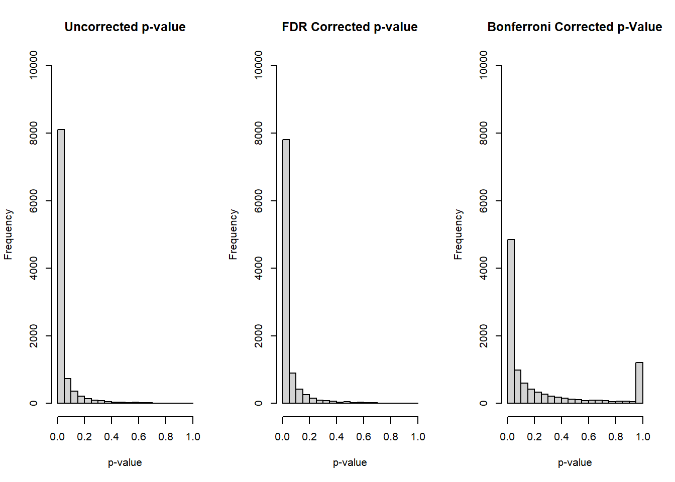
For our alternative scenario we see the approximate behavior we’d expect, where the distribution is strongly concentrated towards lower p-values and is right skewed. One interesting observation is for our Bonferroni correct p-value, where we also see the spike for corrected p-values between 0.95 and 1.0.
Now let’s summarize the power and add it to our results table from above:
orig_marg_pwr <- mean( alt_mat[,paste0('original_p_',1:nhyp)] <= alpha )
fdr_marg_pwr <- mean( alt_mat[,paste0('fdr_p_',1:nhyp)] <= alpha )
bonf_marg_pwr <- mean( alt_mat[,paste0('bonf_p_',1:nhyp)] <= alpha )

res_tab <- cbind(res_tab, 'Power'=c(orig_marg_pwr, fdr_marg_pwr, bonf_marg_pwr))

kbl(res_tab, align='ccc', escape=F) %>%
kable_styling(bootstrap_options = "striped", full_width = F, position = "left")| Marginal T1E | Family-wise T1E | Power | |
|---|---|---|---|
| Uncorrected | 0.0520 | 0.422 | 0.8110 |
| FDR | 0.0054 | 0.050 | 0.7804 |
| Bonferroni | 0.0050 | 0.050 | 0.4844 |
Here we see the trade-offs between our different approaches:
Our uncorrected approach has our desired marginal type I error rate and power, but the family-wise type I error rate is very large.
The FDR has a conservative marginal type I error rate, but achieves the desired \(\alpha\) for our family-wise type I error rate. The power is slightly lower than the uncorrected, but not by much in this case.
The Bonferroni has similar type I error rates as the FDR, but it is far more conservative since its power is only 48.4%.
Let’s just see the results for our study if we up the number of tests to 100 from 10:
# Step 1: set the seed for reproducibility
set.seed(11172020)

# Step 2: define variables of interest (that will be easy to change for different simulations)
nsim <- 1000 # number of simulations
nhyp <- 100 # number of hypothesis tests
alpha <- 0.05 # type I error rate

# set simulation parameters for data:
mean_grp1 <- 0
mean_grp2_null <- 0 # null scenario
mean_grp2_alt <- 10 # alternative scenario
sd_grp1 <- 15
sd_grp2 <- 15
n_grp1 <- 37
n_grp2 <- 37

# Step 3: initialize a matrix to store our results in for each test based on our 3 approaches
null_mat <- matrix(nrow=nsim, ncol=nhyp*3)
colnames( null_mat ) <- c( paste0('original_p_',1:nhyp), paste0('fdr_p_',1:nhyp), paste0('bonf_p_',1:nhyp) )

alt_mat <- null_mat # create alt_mat to save results in for alternative scenario

# Step 4: simulate the trials and hypotheses, store the p-value results
for(i in 1:nsim){
  simdat_grp1 <- matrix( rnorm( n=n_grp1*nhyp, mean=mean_grp1, sd=sd_grp1 ), ncol=nhyp, nrow=n_grp1, byrow=FALSE)
  simdat_grp2 <- matrix( rnorm( n=n_grp2*nhyp, mean=mean_grp2_null, sd=sd_grp2 ), ncol=nhyp, nrow=n_grp2, byrow=FALSE)
  simdat_grp2_alt <- matrix( rnorm( n=n_grp2*nhyp, mean=mean_grp2_alt, sd=sd_grp2 ), ncol=nhyp, nrow=n_grp2, byrow=FALSE)

  # null scenario
  pvec_orig <- sapply( 1:nhyp, function(x) t.test(x=simdat_grp1[,x], y=simdat_grp2[,x])$p.value )
  pvec_fdr <- p.adjust( pvec_orig, method='fdr')
  pvec_bonf <- p.adjust( pvec_orig, method='bonferroni')

  null_mat[i,] <- c(pvec_orig, pvec_fdr, pvec_bonf)

  # alternative scenario
  pvec_orig_alt <- sapply( 1:nhyp, function(x) t.test(x=simdat_grp1[,x], y=simdat_grp2_alt[,x])$p.value )
  pvec_fdr_alt <- p.adjust( pvec_orig_alt, method='fdr')
  pvec_bonf_alt <- p.adjust( pvec_orig_alt, method='bonferroni')

  alt_mat[i,] <- c(pvec_orig_alt, pvec_fdr_alt, pvec_bonf_alt)
}

# Make Table for Results
orig_marg_t1e <- mean( null_mat[,paste0('original_p_',1:nhyp)] <= alpha )
fdr_marg_t1e <- mean( null_mat[,paste0('fdr_p_',1:nhyp)] <= alpha )
bonf_marg_t1e <- mean( null_mat[,paste0('bonf_p_',1:nhyp)] <= alpha )

orig_fw_t1e <- mean( rowSums(null_mat[,paste0('original_p_',1:nhyp)] <= alpha) > 0 )
fdr_fw_t1e <- mean( rowSums(null_mat[,paste0('fdr_p_',1:nhyp)] <= alpha) > 0  )
bonf_fw_t1e <- mean( rowSums(null_mat[,paste0('bonf_p_',1:nhyp)] <= alpha) > 0  )

orig_marg_pwr <- mean( alt_mat[,paste0('original_p_',1:nhyp)] <= alpha )
fdr_marg_pwr <- mean( alt_mat[,paste0('fdr_p_',1:nhyp)] <= alpha )
bonf_marg_pwr <- mean( alt_mat[,paste0('bonf_p_',1:nhyp)] <= alpha )

res_tab <- matrix( c(orig_marg_t1e,fdr_marg_t1e,bonf_marg_t1e, orig_fw_t1e, fdr_fw_t1e, bonf_fw_t1e, orig_marg_pwr, fdr_marg_pwr, bonf_marg_pwr)
                   , ncol=3, byrow=F, dimnames = list(c('Uncorrected','FDR','Bonferroni'), c('Marginal T1E','Family-wise T1E','Power')) )

kbl(res_tab, align='ccc', escape=F) %>%
kable_styling(bootstrap_options = "striped", full_width = F, position = "left")| Marginal T1E | Family-wise T1E | Power | |
|---|---|---|---|
| Uncorrected | 0.05007 | 0.992 | 0.80844 |
| FDR | 0.00042 | 0.039 | 0.77744 |
| Bonferroni | 0.00040 | 0.038 | 0.23273 |
Like almost everything in statistics, there is not a single right answer for how to approach the question of multiple comparisons. However, a few considerations are highlighted below.
Is the study “exploratory” or “confirmatory”? One way to distinguish these ideas is that exploratory research should be hypothesis generating, whereas confirmatory research should have a well-defined hypothesis you are attempting to evaluate. It is possible things fall along this spectrum as well, but this should be identified at the start of the study design and/or data collection process.
Specifying a single primary outcome, a small set of secondary outcomes, and everything else as exploratory outcomes. In this case, the primary outcome would stand on its own, and you wouldn’t have to correct for multiple comparisons. For the secondary outcomes, you may want to correct for multiple comparisons within that set, but it will partly depend on the outcomes in question and the hypotheses being tested. We rarely correct for “exploratory” outcomes in practice.
Instead of the Bonferroni correction, use the Holm (also known as Bonferroni-Holm) correction, which is still conservative but generally has greater power. The challenge with Bonferroni-Holm or FDR, like with many other correction strategies, is it is more complex and it is not easy to generalize for a power/sample size calculation (although you can always do simulation studies!).