This page includes the solutions to the optional practice problems for the given week. If you want to see a version without solutions please click here. Data sets, if needed, are provided on the BIOS 6618 Canvas page for students registered for the course.
This week’s extra practice exercises focus on model/variable selection and examining the potential for influential points.
Exercise 1: Influential Points/Outliers
In our lecture on influential points/outliers we had an example called oildat with 21 observations. The last slide had practice problems that we will examine in further detail here. We can create the data set with the following code:
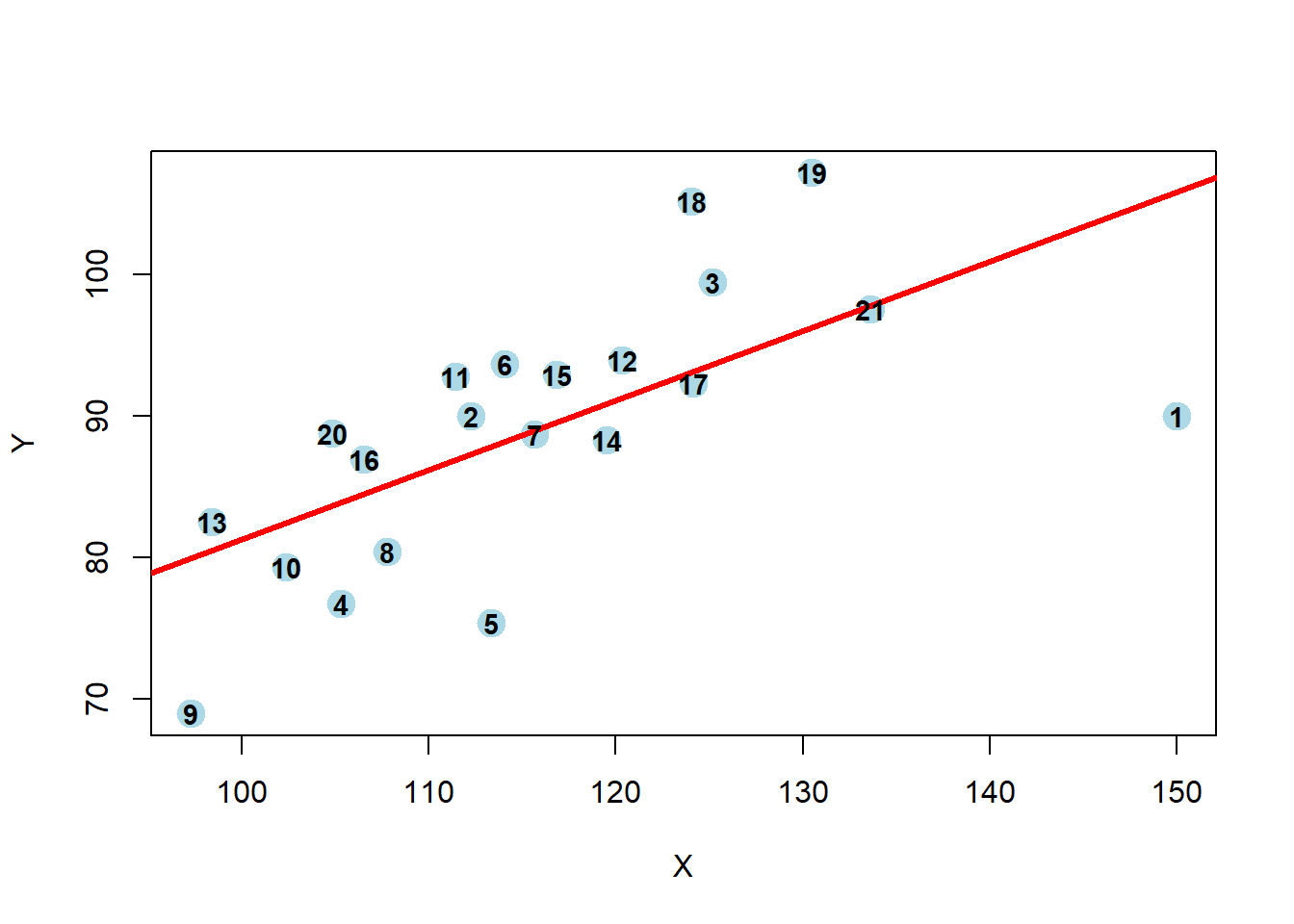
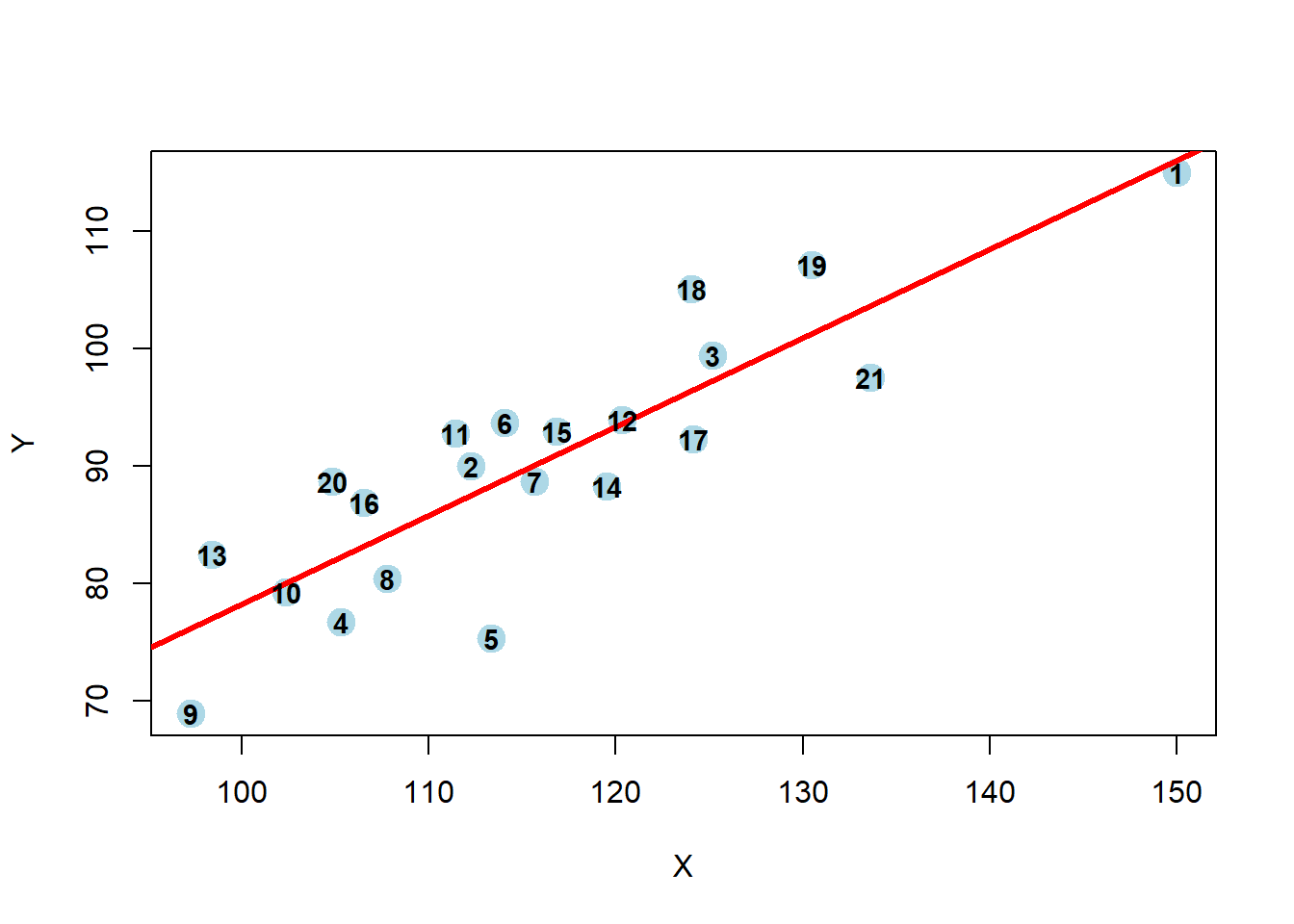
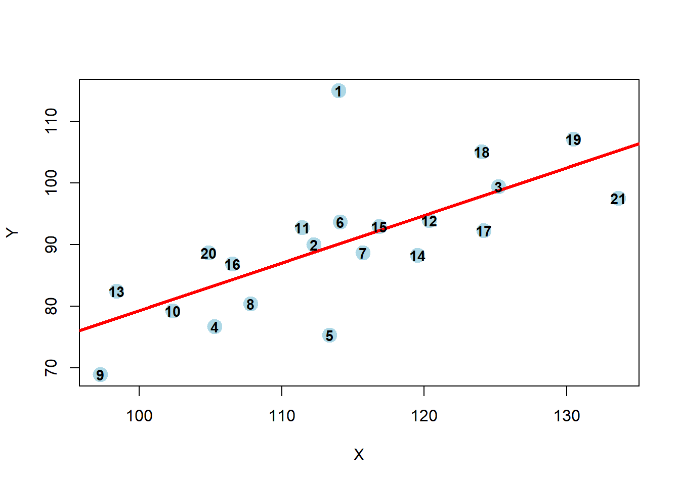
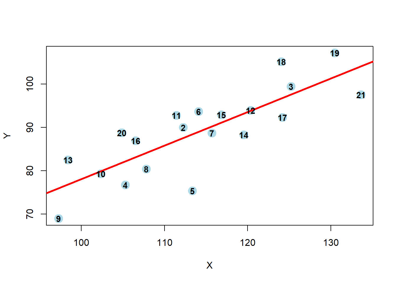
Create a scatterplot of the data with the linear regression fit
Calculate the leverage, jackknife residual, DFFITS, DFBETAS, and Cook’s distance with the corresponding figures from lecture (e.g., using the olsrr package)
1a: Replicating the Lecture Results
Using the observed data, recreate the results from our slides.
Solution:
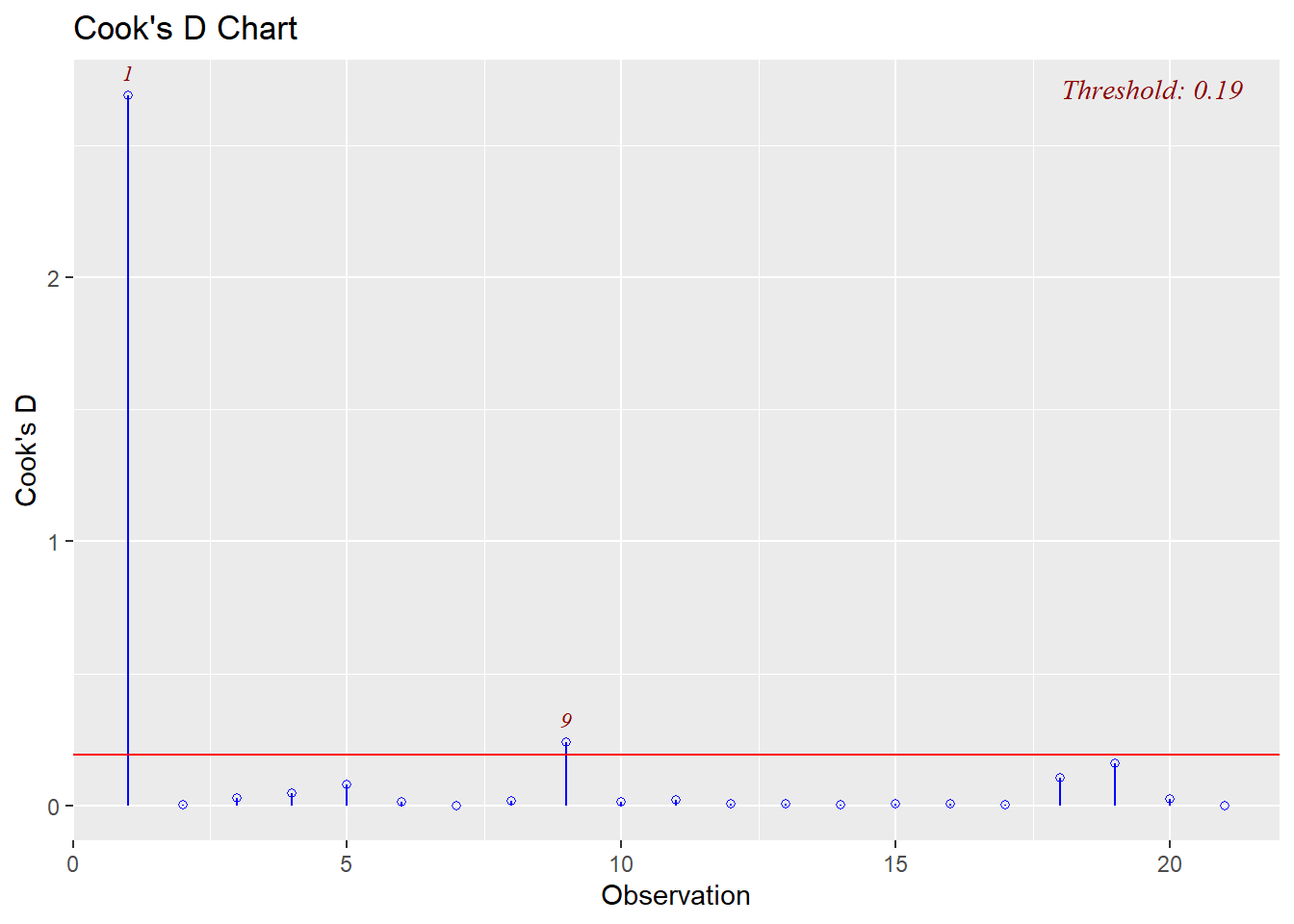
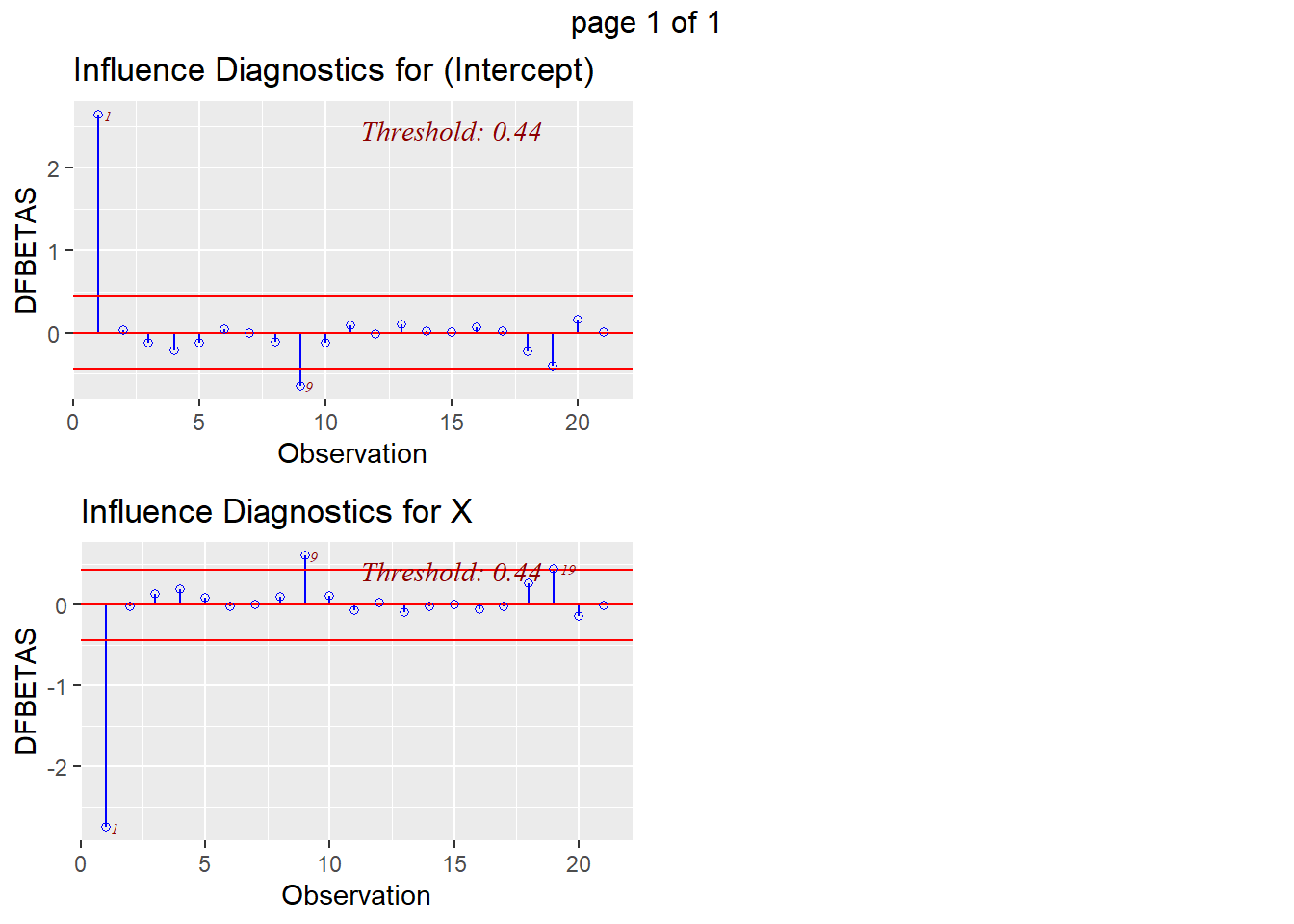
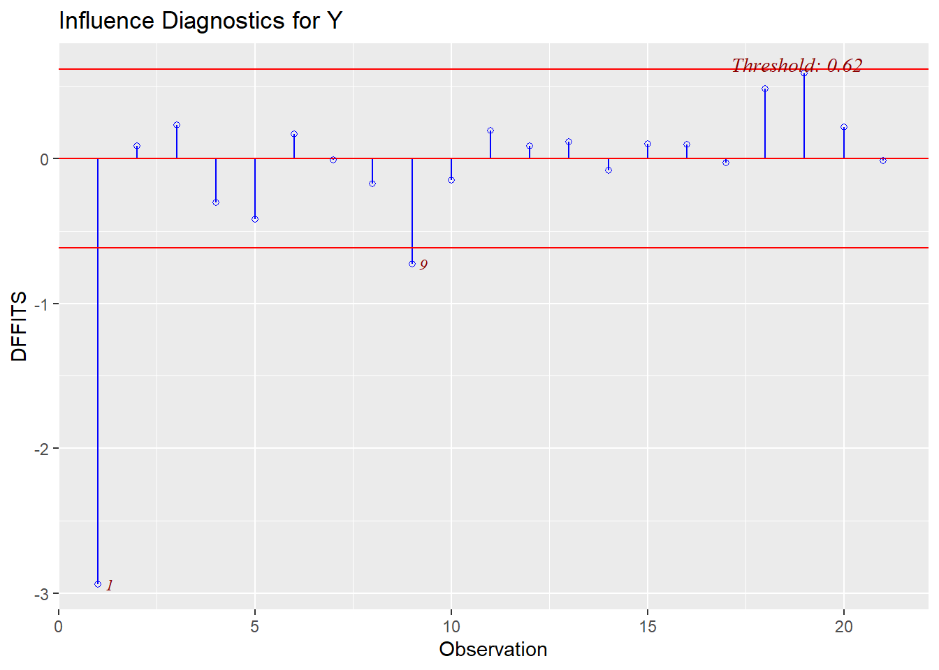
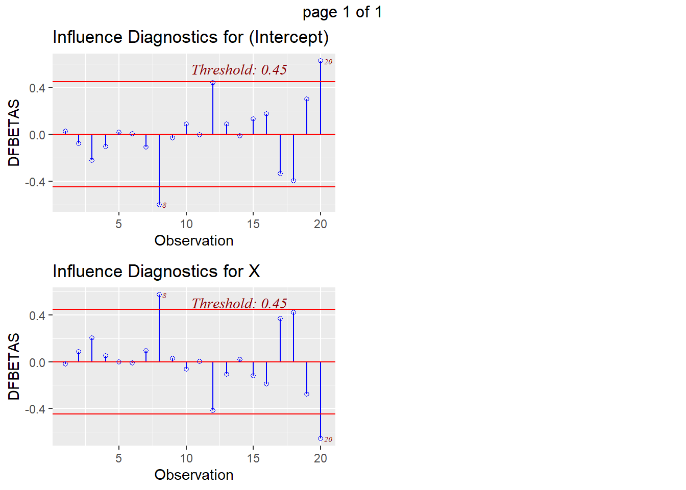
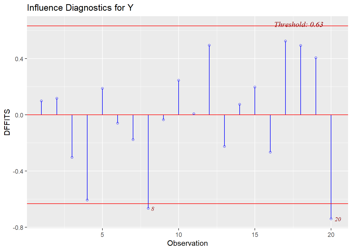
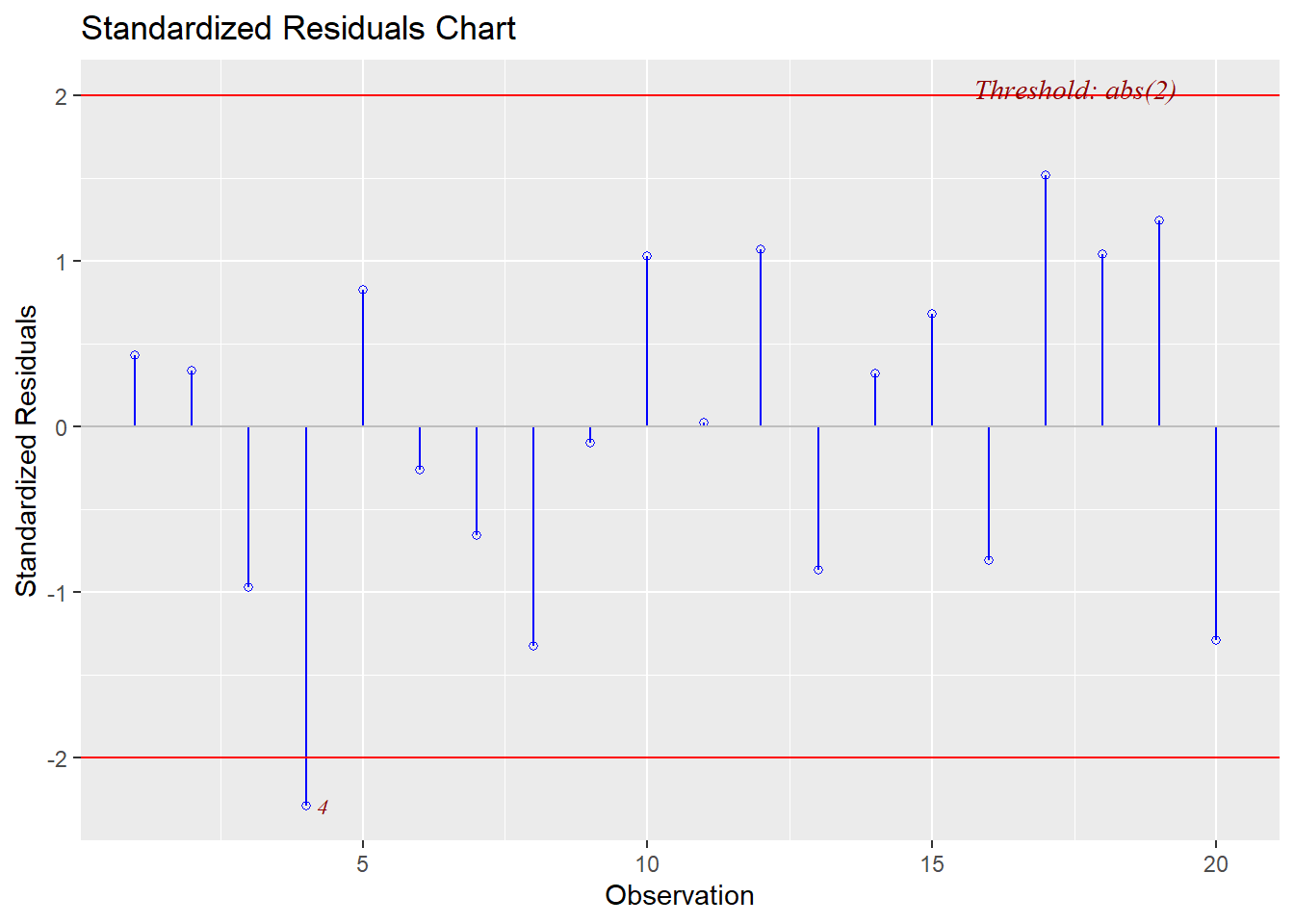
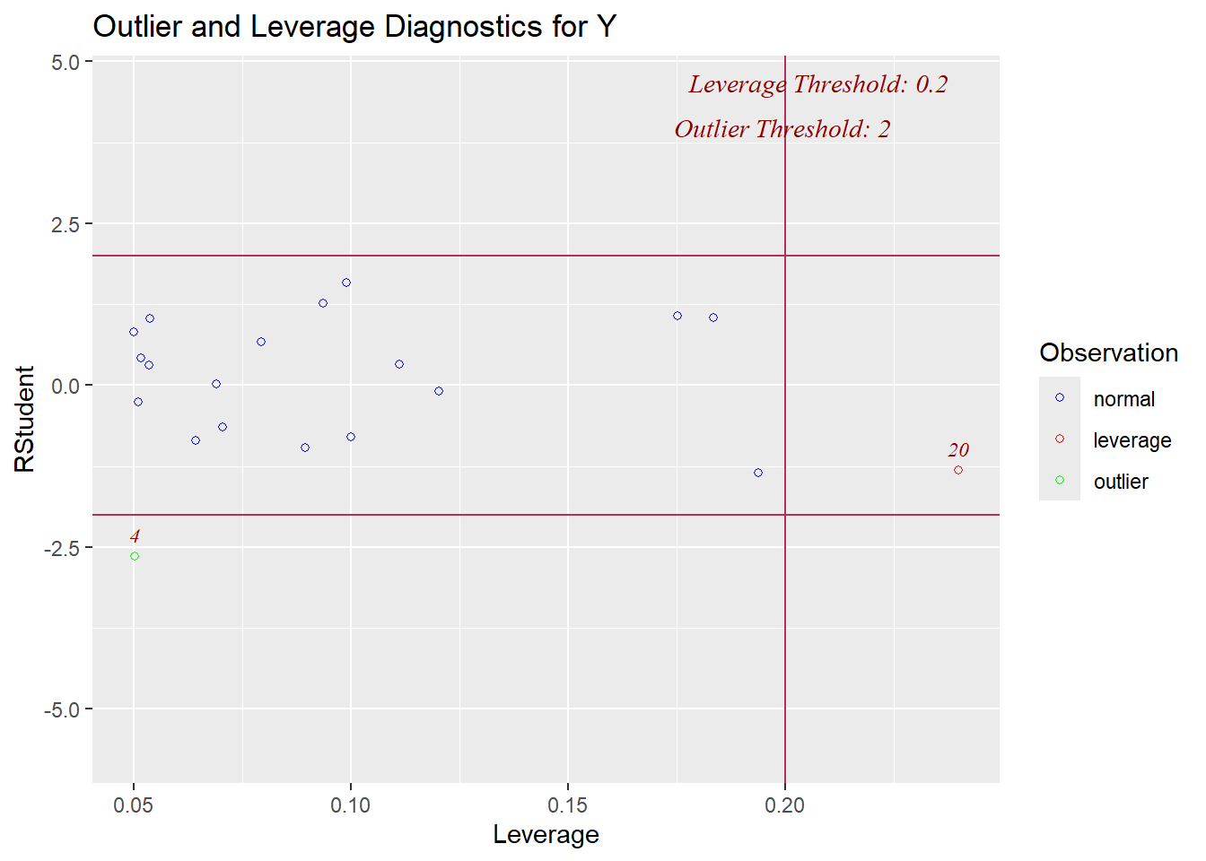
Recall, we have the following thresholds for determining influence, leverage, or outliers:
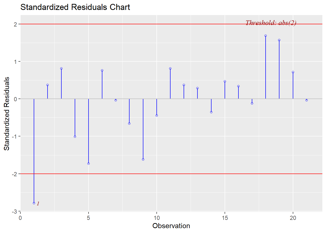
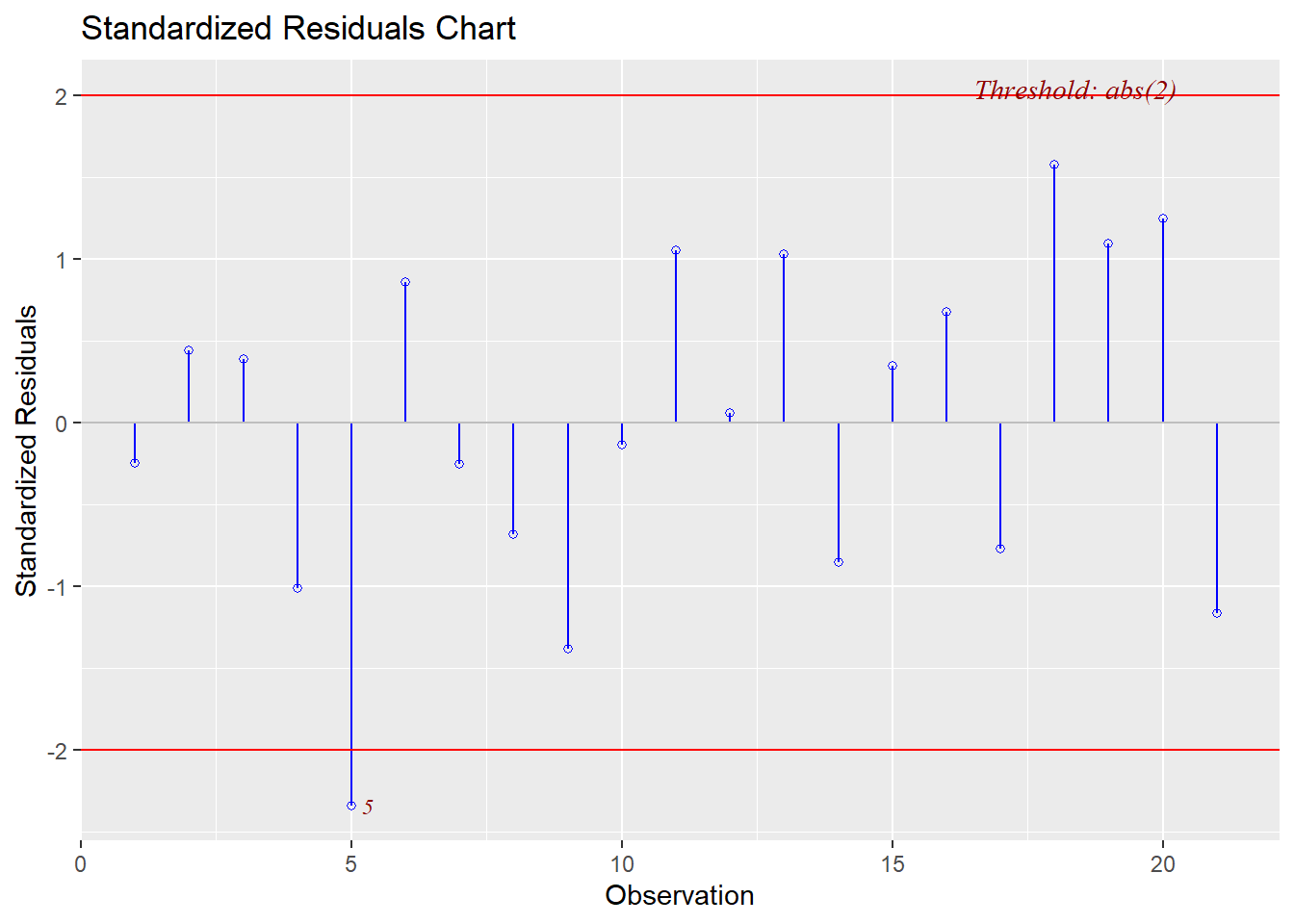
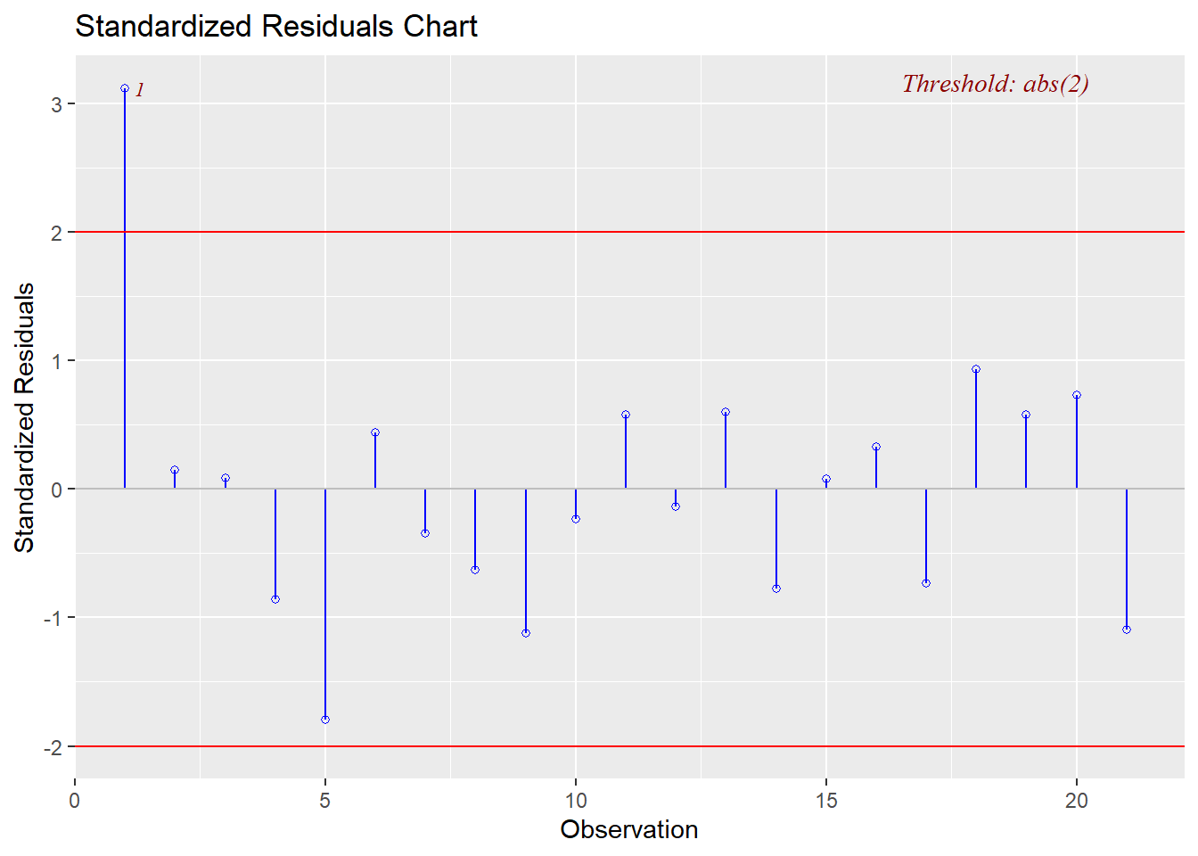
Jackknife Residuals: None are outside the range of \(\pm3\)
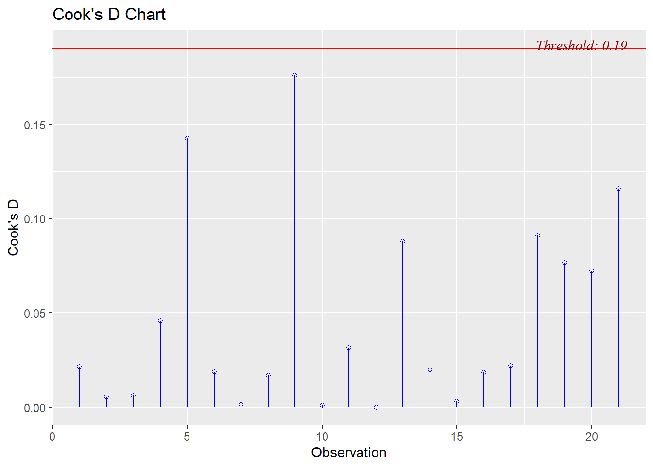
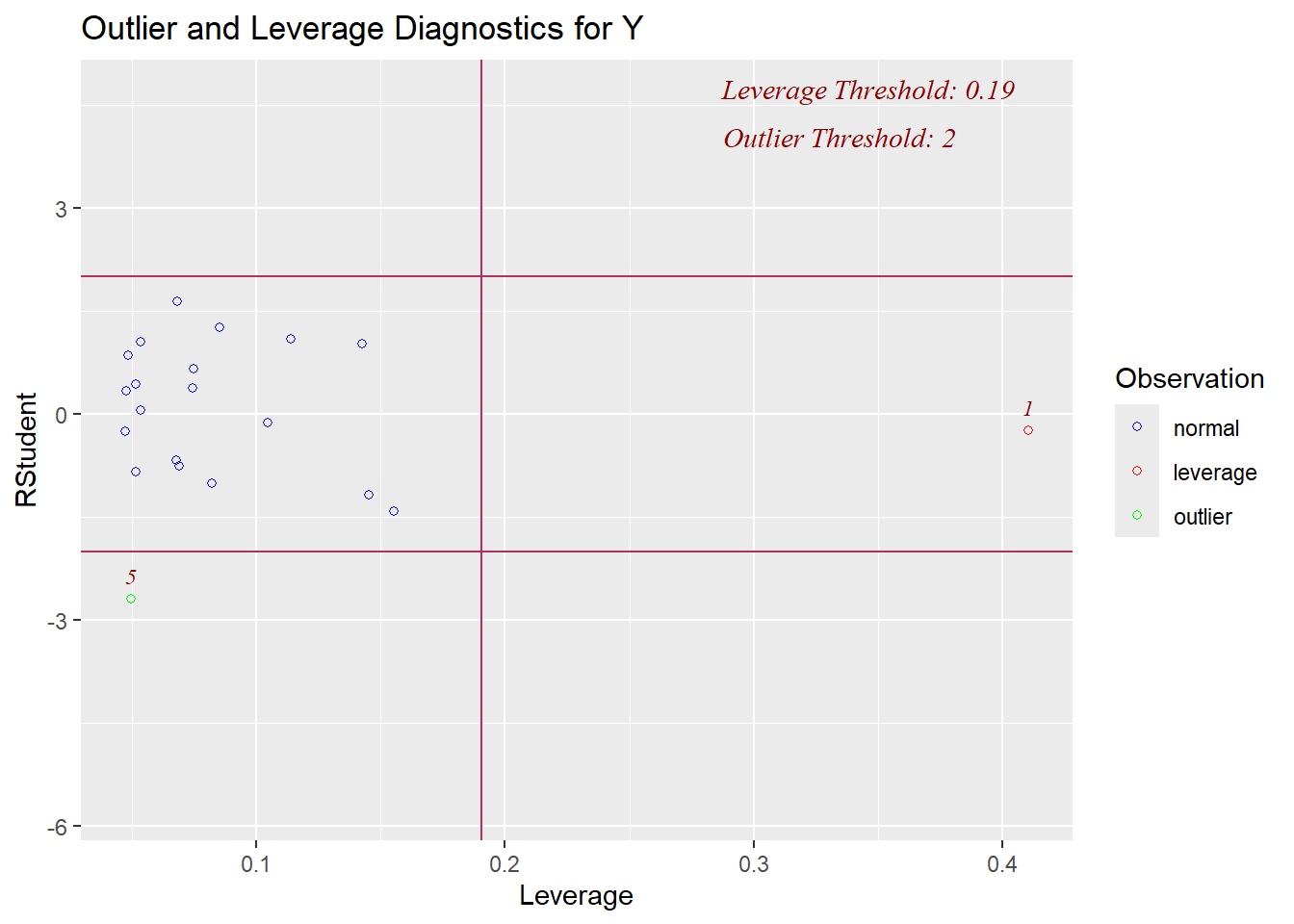
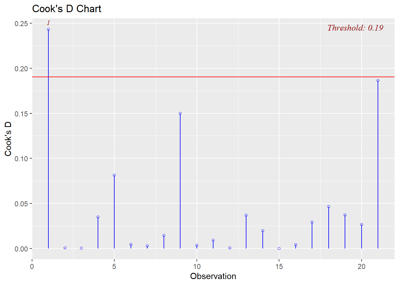
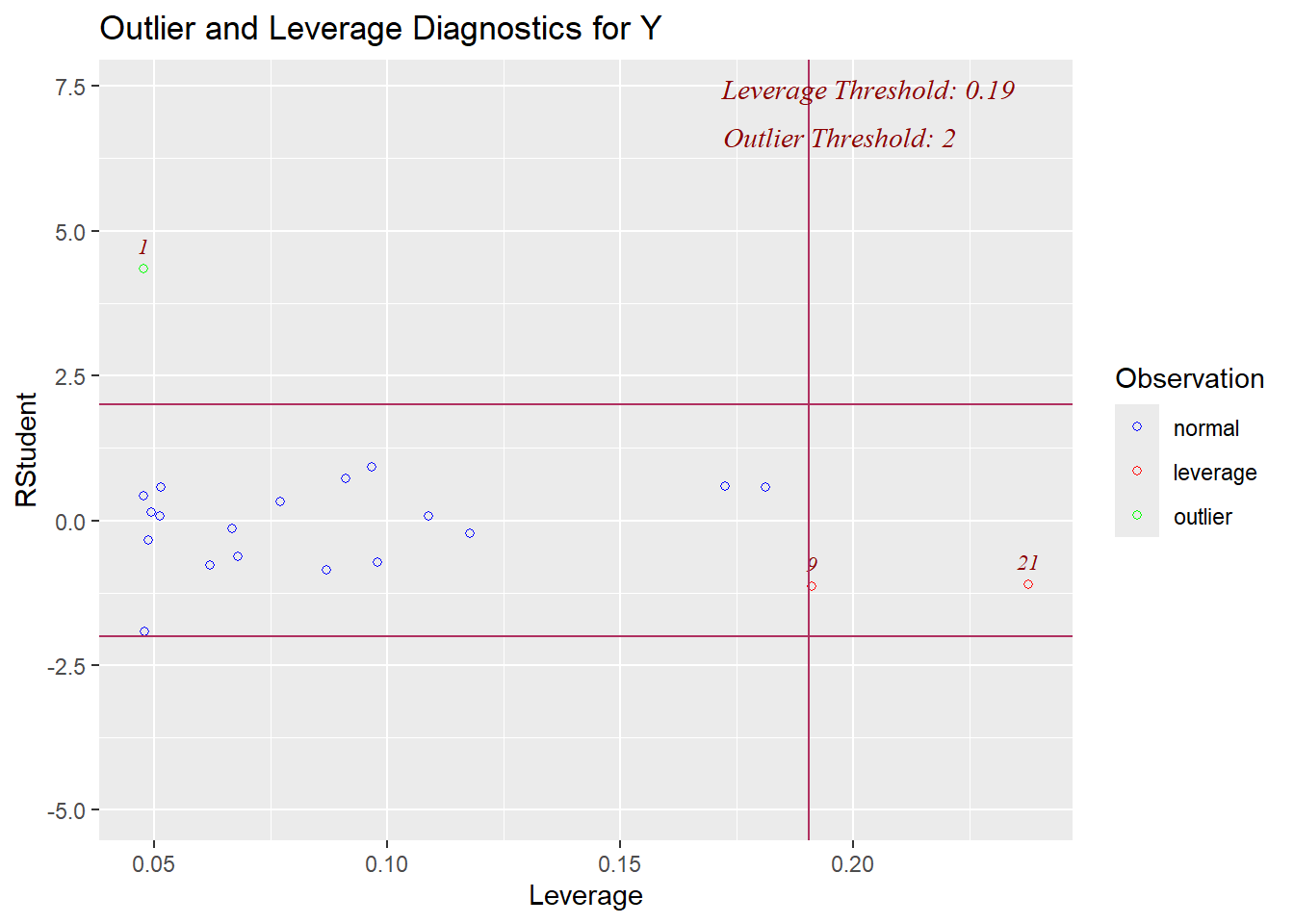
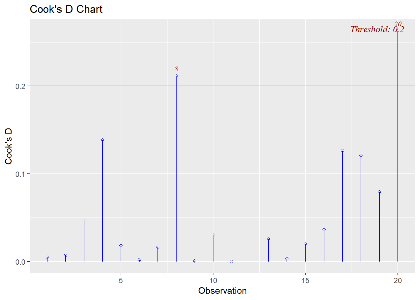
Cook’s Distance: observation 1 has 2.69 > 1 and may be an influential point
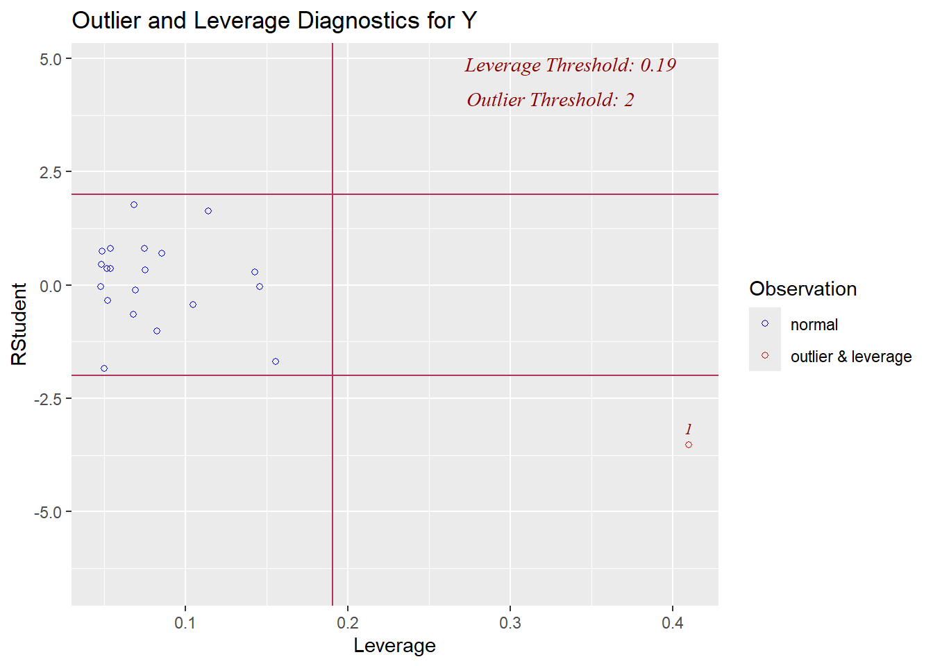
Leverage: observation 1 has 0.41>0.19 and may have high leverage
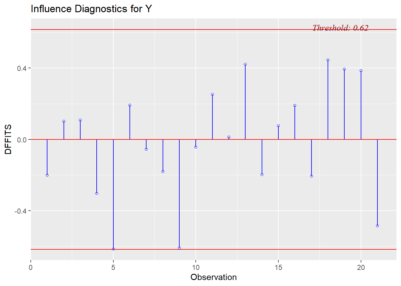
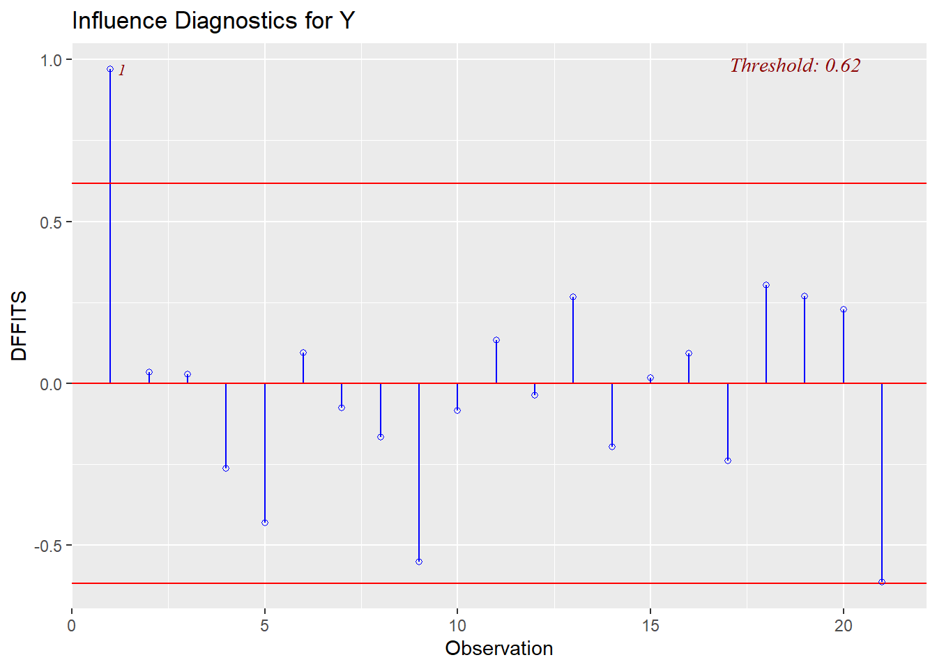
DFFITS: observations 1 and 9 are both larger than our threshold (observation 1 has -2.96 < -0.62; observation 9 has -0.73 < -0.62)
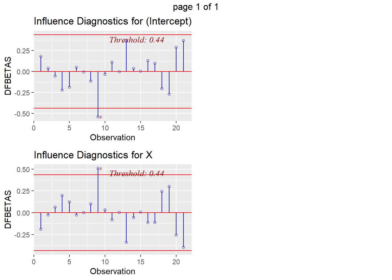
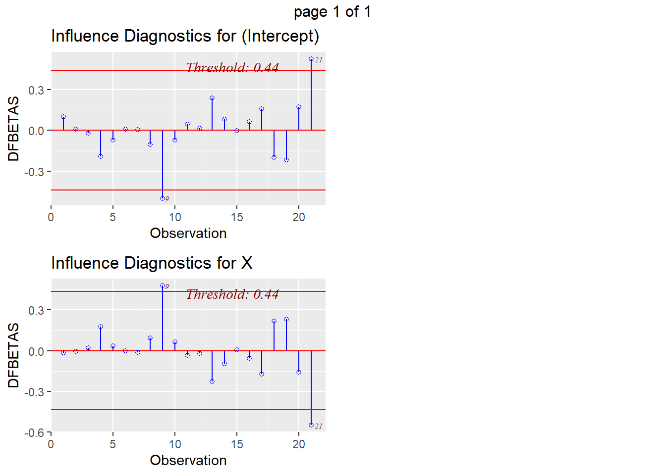
DFBETAS: observation 1 has both the intercept and predictor with large value (intercept has 2.64 > 0.44, predictor has -2.76 < -0.44); observations 9 and 19 also have values indicating potential influence
We can also visualize the evaluation of influence/leverage/outliers (and olsrr will add the thresholds to our plots):
Code
# create plots of data# plot the data with labelsplot(Y~X, col="lightblue",pch=19,cex=2,data=oildat)abline(lm0,col="red",lwd=3)text(Y~X, labels=rownames(oildat),cex=0.9,font=2,data=oildat)
Code
# plot Cook's D (one measure of influence)ols_plot_cooksd_chart(lm0)
Code
# plot DFBETAS (one measure of influence)ols_plot_dfbetas(lm0)
Code
# plot DFFITS (one measure of influence)ols_plot_dffits(lm0)
Code
# Plot standardized residuals (one measure for outliers)ols_plot_resid_stand(lm0)
Code
# Plot outlier and leverage diagnostics plotols_plot_resid_lev(lm0)
This final plot nicely shows that observation 1 may be both an outlier and a leverage point.
1b: Modification 1
Replace first row of data with (X,Y)=(150, 115). Confirm the first observation is not an outlier, has little influence, and has high leverage.
Solution:
Code
# manipulate dataoildat2 <- oildatoildat2[1,] <-c(150,115)# Fit model and calculate summarieslm1 <-lm(Y~X, data=oildat2)jk <-rstandard(lm1)cooksd <-cooks.distance(lm1)leverage <-hatvalues(lm1)dffits_vals <-dffits(lm1)dfbetas_int <-dfbetas(lm1)[,1]dfbetas_X <-dfbetas(lm1)[,2]influence_measures_df2 <-cbind("JKResiduals"= jk, "CooksDistance"=cooksd,"Leverage"= leverage,"DFFITS"=dffits_vals,"DFBETAS_int"=dfbetas_int,"DFBETAS_X"=dfbetas_X)# print influence measures data frameround(influence_measures_df2,2)
For observation 1, specifically, we now see that is has low estimates within our threshold for the jackknife residuals, Cook’s D, DFFITS, and DFBETAS. However, observation 1 still has a high estimate of leverage.
Our plots reflect this change:
Code
# create plots of data# plot the data with labelsplot(Y~X, col="lightblue",pch=19,cex=2,data=oildat2)abline(lm1,col="red",lwd=3)text(Y~X, labels=rownames(oildat2),cex=0.9,font=2,data=oildat2)
Code
# plot Cook's D (one measure of influence)ols_plot_cooksd_chart(lm1)
Code
# plot DFBETAS (one measure of influence)ols_plot_dfbetas(lm1)
Code
# plot DFFITS (one measure of influence)ols_plot_dffits(lm1)
Code
# Plot standardized residuals (one measure for outliers)ols_plot_resid_stand(lm1)
Code
# Plot outlier and leverage diagnostics plotols_plot_resid_lev(lm1)
Unlike the original data (in 1a), we see here that observation 1 is only considered a leverage point (but not an outlier). Interestingly, this change for the 1st observation results in the 5th observation being a potential outlier.
1c: Modification 2
Replace first row of data with (X,Y)=(114, 115). Confirm the first observation is an outlier, has little influence, and has low leverage.
Solution:
Code
# manipulate dataoildat2 <- oildatoildat2[1,] <-c(114,115)# Fit model and calculate summarieslm2 <-lm(Y~X, data=oildat2)jk <-rstandard(lm2)cooksd <-cooks.distance(lm2)leverage <-hatvalues(lm2)dffits_vals <-dffits(lm2)dfbetas_int <-dfbetas(lm2)[,1]dfbetas_X <-dfbetas(lm2)[,2]influence_measures_df3 <-cbind("JKResiduals"= jk, "CooksDistance"=cooksd,"Leverage"= leverage,"DFFITS"=dffits_vals,"DFBETAS_int"=dfbetas_int,"DFBETAS_X"=dfbetas_X)# print influence measures data frameround(influence_measures_df3,2)
For observation 1, specifically, we see it has a jackknife residual >3 (indicating it may be an outlier) and that it generally has little influence and leverage (the exception being its DFFITS is 0.97 > 0.62).
Our plots reflect this change:
Code
# create plots of data# plot the data with labelsplot(Y~X, col="lightblue",pch=19,cex=2,data=oildat2)abline(lm2,col="red",lwd=3)text(Y~X, labels=rownames(oildat2),cex=0.9,font=2,data=oildat2)
Code
# plot Cook's D (one measure of influence)ols_plot_cooksd_chart(lm2)
Code
# plot DFBETAS (one measure of influence)ols_plot_dfbetas(lm2)
Code
# plot DFFITS (one measure of influence)ols_plot_dffits(lm2)
Code
# Plot standardized residuals (one measure for outliers)ols_plot_resid_stand(lm2)
Code
# Plot outlier and leverage diagnostics plotols_plot_resid_lev(lm2)
Unlike the original data (in 1a), we see here that observation 1 is only an outlier but not a leverage point. However, this change in value has led to observations 9 and 21 being potential leverage points.
1d: Modification 3
Remove the first row of data. Confirm there are no outliers, influential points or leverage points.
Solution:
Since we’ve removed a data point, some of our thresholds will change (albeit slightly):
# create plots of data# plot the data with labelsplot(Y~X, col="lightblue",pch=19,cex=2,data=oildat2)abline(lm3,col="red",lwd=3)text(Y~X, labels=rownames(oildat2),cex=0.9,font=2,data=oildat2)
Code
# plot Cook's D (one measure of influence)ols_plot_cooksd_chart(lm3)
Code
# plot DFBETAS (one measure of influence)ols_plot_dfbetas(lm3)
Code
# plot DFFITS (one measure of influence)ols_plot_dffits(lm3)
Code
# Plot standardized residuals (one measure for outliers)ols_plot_resid_stand(lm3)
Code
# Plot outlier and leverage diagnostics plotols_plot_resid_lev(lm3)
By removing the first observation, we see that our resulting diagnostics suggest that most points do not have extreme influence or leverage, and are likely not outliers. However, some values are beyond our thresholds and may not reflect the strong claim that there are definitively no outliers, influential points or leverage points. This also helps to further demonstrate that simply removing a “problem” observation does not necessarily fix everything and can still result in other points becoming potentially concerning.
Exercise 2: Model and Variable Selection for a Real Dataset
We will explore the various model selection and variable selection approaches with the blood storage data set loaded into R using:
Code
dat <-read.csv('../../.data/Blood_Storage.csv')
For our example, we will consider the outcome of preoperative prostate specific antigen (PSA) (PreopPSA) with predictors for age (Age), prostate volume in grams (PVol), tumor volume (TVol as 1=low, 2=medium, 3=extensive), and biopsy Gleason score (bGS as 1=score 0-6, 2=score 7, 3=score 8-10).
2a: Model Selection Approaches
Using all subsets regression, calculate the AIC, AICc, BIC, adjusted R2, and Mallows’ Cp. Identify the optimal model for each approach. Hint: you may need to use expand.grid, for loops, or other manual coding to generate all possible models and calculate each summary.
Solution:
We can use expand.grid to generate indicators for all variables and then fit each model in a for loop and save all generated summaries. We will also want to convert our categorical variables from numeric to a factor or text string so R does not treat them as continuous predictors and create a new dataset with records with complete data for our outcome/predictors:
Code
# modify categorical variables with multiple categoriesdat$TVol <-factor(dat$TVol, levels=c(1,2,3), labels=c('Low','Medium','Extensive'))dat$bGS <-factor(dat$bGS, levels=c(1,2,3), labels=c('0-6','7','8-10'))# reduce data to complete casesdatc <- dat[complete.cases(dat[,c('PreopPSA','Age','PVol','TVol','bGS')]),]# create data frame with all combinations of predictorsall_subsets <-expand.grid(Age=c(0,1), PVol=c(0,1),TVol=c(0,1),bGS=c(0,1))# create object to save results inres_mat <- all_subsetsres_mat[,c('aic','aicc','bic','r2','cp')] <-NA# calculate full model with all predictors to save MSE for use in Cp calculationfull_mod <-lm(PreopPSA ~ Age + PVol + TVol + bGS, data=datc)full_mse <-sum(residuals(full_mod)^2) / (nrow(datc) -6-1) # calculate MSE for full model# loop through each combination and save resultsfor( i in1:nrow(all_subsets)){ rhs_lm <-paste0( colnames(all_subsets)[which(all_subsets[i,]==1)], collapse ='+') # automatically extract included variables to place onto right hand side of lm() equationif( rhs_lm =='' ){ lm_i <-lm( PreopPSA ~1, data=datc ) }else{ lm_i <-lm( as.formula(paste0('PreopPSA ~ ', rhs_lm)), data=datc ) } res_mat[i,'aic'] <-AIC(lm_i, k=2) numpred <-length(coef(lm_i))-1# calculate the number of predictors to use for calculation of AICc res_mat[i,'aicc'] <-AIC(lm_i, k=2) + (2*numpred^2+2*numpred) / (nrow(datc) - numpred -1) res_mat[i,'bic'] <-BIC(lm_i) res_mat[i,'r2'] <-summary(lm_i)$adj.r.squared res_mat[i,'cp'] <- ( sum(residuals(lm_i)^2) / full_mse) - (nrow(datc) -2*(numpred+1))}round(res_mat,3)
The results generally agree that a model with everything except age is likely optimal:
AIC and AICc are both minimized for the full model, however the difference between this and the model without age is less than 2, suggesting the more parsimonious model may be more appropriate.
BIC is minimized for model excluding only age. We might also consider the model with just PVol and TVol (model 7) since its BIC is only 1.015 larger, but the model is more parsimonious.
Our adjusted \(R^2\) is technically maximized for the full model, but the improvement is not large relative to the model excluding age (i.e., 21.1% versus 20.3% of variability explained).
Mallows’ Cp is fairly small for the model excluding age relative to the full model, whereas most other models have a much larger values.
2b: Variable Selection Approaches
Identify the best model using forward selection, backward selection, and stepwise selection based on BIC.
In this example, all four approaches based on BIC for automatic selection agree that the model with all predictors except Age should be used.
2c: Picking a Model
Based on your results from the prior questions, what model would you propose to use in modeling PSA?
Solution:
In this example, most approaches seemed to indicate that the model with PVol, TVol, and bGS should be used. In other words, only Age would be excluded from the model. If we had more context, we might choose a different model, but the evidence from both variable and model selection approaches in this specific example seems to indicate this would be the most parsimonious model.
Exercise 3: A Simulation Study for Model Selection Approaches
With our real dataset in Exercise 2 we cannot be sure what the “true” model would be. While we were fortunate most approaches were agreement for the “optimal” model, it rarely works this nicely. One way we can evaluate the performance of each of these methods is to simulate a scenario with a mixture of null and non-null predictors and see how often each variable is chosen for the model.
While we can simulate increasingly complex models (e.g., interactions, polynomial terms, etc.), we will simulate a data set of \(n=200\) with 20 independent predictors (i.e., no true correlation between any two predictors):
5 continuous simulated from \(N(0,1)\), where 2 are null and 3 have effect sizes of 2, 1, and 0.5
5 binary simulated with \(p=0.5\), where 2 are null and 3 have effect sizes of 2, 1, and 0.5
Via simulation, we will be able to draw conclusions about (1) whether the strength of the effect matters or (2) if continuous or binary predictors have differences.
Use the following code to generate the data for each simulation iteration assuming an intercept of -2 and \(\epsilon \sim N(0,5)\) (you’ll have to incorporate a seed, etc. in your own simulations):
Simulate the data set and fit the full model 1,000 times using set.seed(12521). Summarize the power/type I error for each variable.
Solution:
For this simulation we will create a matrix to store if the resulting p-values are less than 0.05 for all predictors and the intercept, then summarize the proportion of simulations where a significant p-value was found:
Code
set.seed(12521)n <-200nsim <-1000power_mat <-matrix(nrow=nsim, ncol=11,dimnames =list(1:nsim, paste0('beta',0:10))) # create matrix to save results in, with additional column for interceptfor(j in1:nsim){ Xc <-matrix( rnorm(n=200*5, mean=0, sd=1), ncol=5) # simulate continuous predictors Xb <-matrix( rbinom(n=200*5, size=1, prob=0.5), ncol=5) # simulate binary predictors simdat <-as.data.frame( cbind(Xc, Xb) ) # create data frame of predictors to add outcome to simdat$Y <--2+2*simdat$V1 +1*simdat$V2 +0.5*simdat$V3 +2*simdat$V6 +1*simdat$V7 +0.5*simdat$V8 +rnorm(n=n, mean=0, sd=5) lmj <-lm(Y ~ ., data=simdat) power_mat[j,] <-summary(lmj)$coefficients[,'Pr(>|t|)'] <0.05# save if p-values are less than 0.05}# calculate powercolMeans(power_mat)
From our output, we see that we have 99.9% power for \(\beta_1 = 2\), 79.4% power when the continuous predictor effect size decreases to \(\beta_2 = 1\), and only 30.1% when \(\beta_3=0.5\). For our categorical predictors there is lower power with 78.9% for \(\beta_{6} = 2\), 30.6% for \(\beta_{7}=1\), and 12.2% for \(\beta_{8}=0.5\). Our covariates with no effect (i.e., \(\beta_i = 0\)) are generally around 5%, and the intercept has 63.0% power.
3b: The “Best” Model
Simulate the data set 1,000 times using set.seed(12521). For each data set identify the variables included in the optimal model for AIC, AICc, BIC, adjusted R2, backward selection, forward selection, stepwise selection from the null model, and stepwise selection from the full model. For model selection criteria, select the model that minimizes the criterion (i.e., we will ignore if other models might have fewer predictors but only a slightly larger criterion for sake of automating the simulation). For automatic selection models use BIC.
Summarize both how often the “true” model is selected from each approach (i.e., with the 3 continuous and 3 categorical predictors that are non-null), as well as how often each variable was selected more generally. Does one approach seem better overall? On average?
Solution:
With 10 predictors, there are \(2 ^ {10} = 1024\) possible models. In order to manually fit this many models for each simulation, it will likely take more time than our previous simulations from class. We can help streamline the process by writing a function to apply for each simulated data set and return the desired information for the optimally identified model:
Code
# Write function based on exercise 2 to apply to each simulated data setoptimal_model <-function(datopt, simnum){## Function to calculate AIC, AICc, BIC, adjusted R^2, and automatic selection models based on BIC # datopt: dataframe with outcome Y and all other columns for predictors# simnum: simulation number for tracking purposes# create data frame with all combinations of predictors all_subsets <-expand.grid( rep(list(c(0,1)), ncol(datopt)-1) )colnames(all_subsets) <-paste0('V',1:(ncol(datopt)-1))# create object to save results in res_mat <- all_subsets res_mat[,c('aic','aicc','bic','r2')] <-NA# loop through each combination and save resultsfor( i in1:nrow(all_subsets)){ rhs_lm <-paste0( colnames(all_subsets)[which(all_subsets[i,]==1)], collapse ='+') # automatically extract included variables to place onto right hand side of lm() equationif( rhs_lm =='' ){ lm_i <-lm( Y ~1, data=datopt ) }else{ lm_i <-lm( as.formula(paste0('Y ~ ', rhs_lm)), data=datopt ) } res_mat[i,'aic'] <-AIC(lm_i, k=2) numpred <-length(coef(lm_i))-1# calculate the number of predictors to use for calculation of AICc res_mat[i,'aicc'] <-AIC(lm_i, k=2) + (2*numpred^2+2*numpred) / (nrow(datopt) - numpred -1) res_mat[i,'bic'] <-BIC(lm_i) res_mat[i,'r2'] <-summary(lm_i)$adj.r.squared } full_mod <-lm(Y ~ ., data=datopt) null_mod <-lm(Y ~1, data=datopt) n <-nrow(datopt)# backward selection backward <-step(full_mod, direction='backward', k=log(n), trace=0)# forward selection forward <-step(null_mod, direction='forward',scope =as.formula(paste0('~ ', paste0('V',1:(ncol(datopt)-1), collapse='+'))),k=log(n),trace=0)# stepwise selection starting with null model stepwise_null <-step(null_mod, direction='both',scope =as.formula(paste0('~ ', paste0('V',1:(ncol(datopt)-1), collapse='+'))),k=log(n),trace=0)# stepwise selection starting with full model stepwise_full <-step(full_mod, direction='both',k=log(n),trace=0)# collect results to return aic_opt <- res_mat[which( res_mat$aic ==min(res_mat$aic)),paste0('V',1:10)] aicc_opt <- res_mat[which( res_mat$aicc ==min(res_mat$aicc)),paste0('V',1:10)] bic_opt <- res_mat[which( res_mat$bic ==min(res_mat$bic)),paste0('V',1:10)] r2_opt <- res_mat[which( res_mat$r2 ==max(res_mat$r2)),paste0('V',1:10)] back_opt <-paste0('V',1:10) %in%names(backward$coefficients) fw_opt <-paste0('V',1:10) %in%names(forward$coefficients) stepnull_opt <-paste0('V',1:10) %in%names(stepwise_null$coefficients) stepfull_opt <-paste0('V',1:10) %in%names(stepwise_full$coefficients) res_ret <-cbind(data.frame( simnum = simnum, method =c('aic','aicc','bic','r2','forward','backward','stepwise_null','stepwise_full')),rbind( aic_opt, aicc_opt, bic_opt, r2_opt, back_opt, fw_opt, stepnull_opt, stepfull_opt) )}
Now, with a function to implement the identification of the optimal model, we can implement our simulation:
With our 1000 simulation results, we can summarize the answer to our question by variable and for the overall model. For the proportion of times each variable was included in the model we see:
Code
library(doBy)perc_mean <-function(x) round(100*mean(x), 1) # create function to present % of simulations including variablesummaryBy( V1 + V2 + V3 + V4 + V5 + V6 + V7 + V8 + V9 + V10 ~ method, data=resj, FUN=perc_mean)
We see a trade-off, where AIC, AICc, and the adjusted \(R^2\) have higher rates of including variables. This is true both for those which have an effect of 2, 1, or 0.5, as well as the null variables (V4, V5, V9, V10).
In contrast, BIC and the automatic procedures based on BIC are all fairly similar. While they almost always detect V1, the have lower rates of detecting V2, V3, V6, V7, and V8.
These results suggest that continuous variables are more often identified than categorical predictors, which makes sense given that continuous predictors have more information contained in their values (since they aren’t restricted to be 0/1). Further, the adjusted \(R^2\) is overly optimistic and picks null variables at a much higher rate, with the AIC and AICc being similar optimistic.
We can also summarize the proportion of models each approach identified that perfectly aligned with our true data generating scenario:
We see that the true model is never identified across any simulations. This may be due to a few different contributing factors:
Each simulation is based on an underlying truth, but by chance each simulation can differ from the truth.
From our power calculation, we know that those with 1 and 0.5 effect sizes have lower power. If we designed a simulation where all non-null coefficients had at least 80% power, we likely would see more scenarios that correctly identified the true model.
However, this is useful to recall the old adage by George Box, a British statistician, that “all models are wrong, but some are useful.” While no single approach guarantees the “true” data generating model, each likely is useful for the given sample and we can use our variable-specific results to identify the method(s) that might reflect our comfort level with including null variables (e.g., AIC) or excluding non-null variables with lower effect sizes (e.g., BIC).
Source Code
---title: "Week 12 Practice Problems: Solutions"author: name: Alex Kaizer roles: "Instructor" affiliation: University of Colorado-Anschutz Medical Campustoc: truetoc_float: truetoc-location: leftformat: html: code-fold: show code-overflow: wrap code-tools: true---```{r, echo=F, message=F, warning=F}library(kableExtra)library(dplyr)```This page includes the solutions to the optional practice problems for the given week. If you want to see a version [without solutions please click here](/labs/prac12/index.qmd). Data sets, if needed, are provided on the BIOS 6618 Canvas page for students registered for the course.This week's extra practice exercises focus on model/variable selection and examining the potential for influential points.# Exercise 1: Influential Points/OutliersIn our [lecture on influential points/outliers](https://www.youtube.com/watch?v=3XUo2b38e6E) we had an example called `oildat` with 21 observations. The last slide had practice problems that we will examine in further detail here. We can create the data set with the following code:```{r}oildat <-data.frame(X =c(150,112.26,125.2,105.31,113.35,114.08,115.68,107.8,97.27,102.35,111.44,120.34,98.4,119.52,116.84,106.52,124.16,124.04,130.47,104.86,133.61),Y =c(90,90.01,99.47,76.76,75.36,93.7,88.72,80.41,68.96,79.33,92.79,93.98,82.51,88.31,92.95,86.93,92.31,105.15,107.19,88.75,97.54))```For each scenario, complete the following:1. Create a scatterplot of the data with the linear regression fit2. Calculate the leverage, jackknife residual, DFFITS, DFBETAS, and Cook's distance with the corresponding figures from lecture (e.g., using the `olsrr` package)## 1a: Replicating the Lecture ResultsUsing the observed data, recreate the results from our slides. **Solution:**Recall, we have the following thresholds for determining influence, leverage, or outliers:* Leverage: $2(p+1)/n=2(2)/21=0.19$* Jackknife Residual: $\pm 3$; $\pm 4$* DDFITS: $\pm 2\sqrt{(p+1)/n}=2\sqrt{2/21}=\pm0.62$* DFBETAS: $\pm 2/\sqrt{n} = 2 /\sqrt{21} = 0.44$* Cook's Distance: $d_i>1.0$```{r, message=F, warning=F}library(olsrr) # load package for visualizations# Fit model and calculate summarieslm0 <-lm(Y~X, data=oildat)jk <-rstandard(lm0)cooksd <-cooks.distance(lm0)leverage <-hatvalues(lm0)dffits_vals <-dffits(lm0)dfbetas_int <-dfbetas(lm0)[,1]dfbetas_X <-dfbetas(lm0)[,2]influence_measures_df <-cbind("JKResiduals"= jk, "CooksDistance"=cooksd,"Leverage"= leverage,"DFFITS"=dffits_vals,"DFBETAS_int"=dfbetas_int,"DFBETAS_X"=dfbetas_X)# print influence measures data frameround(influence_measures_df,2)```In our summaries we see the following:* Jackknife Residuals: None are outside the range of $\pm3$* Cook's Distance: observation 1 has 2.69 > 1 and may be an influential point* Leverage: observation 1 has 0.41>0.19 and may have high leverage* DFFITS: observations 1 and 9 are both larger than our threshold (observation 1 has -2.96 < -0.62; observation 9 has -0.73 < -0.62)* DFBETAS: observation 1 has both the intercept and predictor with large value (intercept has 2.64 > 0.44, predictor has -2.76 < -0.44); observations 9 and 19 also have values indicating potential influenceWe can also visualize the evaluation of influence/leverage/outliers (and `olsrr` will add the thresholds to our plots):```{r}# create plots of data# plot the data with labelsplot(Y~X, col="lightblue",pch=19,cex=2,data=oildat)abline(lm0,col="red",lwd=3)text(Y~X, labels=rownames(oildat),cex=0.9,font=2,data=oildat)# plot Cook's D (one measure of influence)ols_plot_cooksd_chart(lm0)# plot DFBETAS (one measure of influence)ols_plot_dfbetas(lm0)# plot DFFITS (one measure of influence)ols_plot_dffits(lm0)# Plot standardized residuals (one measure for outliers)ols_plot_resid_stand(lm0)# Plot outlier and leverage diagnostics plotols_plot_resid_lev(lm0)```This final plot nicely shows that observation 1 may be both an outlier and a leverage point. ## 1b: Modification 1Replace first row of data with (X,Y)=(150, 115). Confirm the first observation is not an outlier, has little influence, and has high leverage.**Solution:**```{r, message=F, warning=F}# manipulate dataoildat2 <- oildatoildat2[1,] <-c(150,115)# Fit model and calculate summarieslm1 <-lm(Y~X, data=oildat2)jk <-rstandard(lm1)cooksd <-cooks.distance(lm1)leverage <-hatvalues(lm1)dffits_vals <-dffits(lm1)dfbetas_int <-dfbetas(lm1)[,1]dfbetas_X <-dfbetas(lm1)[,2]influence_measures_df2 <-cbind("JKResiduals"= jk, "CooksDistance"=cooksd,"Leverage"= leverage,"DFFITS"=dffits_vals,"DFBETAS_int"=dfbetas_int,"DFBETAS_X"=dfbetas_X)# print influence measures data frameround(influence_measures_df2,2)```For observation 1, specifically, we now see that is has low estimates within our threshold for the jackknife residuals, Cook's D, DFFITS, and DFBETAS. However, observation 1 still has a high estimate of leverage.Our plots reflect this change:```{r}# create plots of data# plot the data with labelsplot(Y~X, col="lightblue",pch=19,cex=2,data=oildat2)abline(lm1,col="red",lwd=3)text(Y~X, labels=rownames(oildat2),cex=0.9,font=2,data=oildat2)# plot Cook's D (one measure of influence)ols_plot_cooksd_chart(lm1)# plot DFBETAS (one measure of influence)ols_plot_dfbetas(lm1)# plot DFFITS (one measure of influence)ols_plot_dffits(lm1)# Plot standardized residuals (one measure for outliers)ols_plot_resid_stand(lm1)# Plot outlier and leverage diagnostics plotols_plot_resid_lev(lm1)```Unlike the original data (in **1a**), we see here that observation 1 is only considered a leverage point (but not an outlier). Interestingly, this change for the 1st observation results in the 5th observation being a potential outlier.## 1c: Modification 2Replace first row of data with (X,Y)=(114, 115). Confirm the first observation is an outlier, has little influence, and has low leverage.**Solution:**```{r, message=F, warning=F}# manipulate dataoildat2 <- oildatoildat2[1,] <-c(114,115)# Fit model and calculate summarieslm2 <-lm(Y~X, data=oildat2)jk <-rstandard(lm2)cooksd <-cooks.distance(lm2)leverage <-hatvalues(lm2)dffits_vals <-dffits(lm2)dfbetas_int <-dfbetas(lm2)[,1]dfbetas_X <-dfbetas(lm2)[,2]influence_measures_df3 <-cbind("JKResiduals"= jk, "CooksDistance"=cooksd,"Leverage"= leverage,"DFFITS"=dffits_vals,"DFBETAS_int"=dfbetas_int,"DFBETAS_X"=dfbetas_X)# print influence measures data frameround(influence_measures_df3,2)```For observation 1, specifically, we see it has a jackknife residual >3 (indicating it may be an outlier) and that it generally has little influence and leverage (the exception being its DFFITS is 0.97 > 0.62).Our plots reflect this change:```{r}# create plots of data# plot the data with labelsplot(Y~X, col="lightblue",pch=19,cex=2,data=oildat2)abline(lm2,col="red",lwd=3)text(Y~X, labels=rownames(oildat2),cex=0.9,font=2,data=oildat2)# plot Cook's D (one measure of influence)ols_plot_cooksd_chart(lm2)# plot DFBETAS (one measure of influence)ols_plot_dfbetas(lm2)# plot DFFITS (one measure of influence)ols_plot_dffits(lm2)# Plot standardized residuals (one measure for outliers)ols_plot_resid_stand(lm2)# Plot outlier and leverage diagnostics plotols_plot_resid_lev(lm2)```Unlike the original data (in **1a**), we see here that observation 1 is only an outlier but not a leverage point. However, this change in value has led to observations 9 and 21 being potential leverage points.## 1d: Modification 3Remove the first row of data. Confirm there are no outliers, influential points or leverage points.**Solution:**Since we've removed a data point, some of our thresholds will change (albeit slightly):* Leverage: $2(p+1)/n=2(2)/20=0.20$* Jackknife Residual: $\pm 3$; $\pm 4$* DDFITS: $\pm 2\sqrt{(p+1)/n}=2\sqrt{2/20}=\pm0.63$* DFBETAS: $\pm 2/\sqrt{n} = 2 /\sqrt{20} = 0.45$* Cook's Distance: $d_i>1.0$```{r, message=F, warning=F}# manipulate dataoildat2 <- oildat[2:21,] # remove 1st observation# Fit model and calculate summarieslm3 <-lm(Y~X, data=oildat2)jk <-rstandard(lm3)cooksd <-cooks.distance(lm3)leverage <-hatvalues(lm3)dffits_vals <-dffits(lm3)dfbetas_int <-dfbetas(lm3)[,1]dfbetas_X <-dfbetas(lm3)[,2]influence_measures_df3 <-cbind("JKResiduals"= jk, "CooksDistance"=cooksd,"Leverage"= leverage,"DFFITS"=dffits_vals,"DFBETAS_int"=dfbetas_int,"DFBETAS_X"=dfbetas_X)# print influence measures data frameround(influence_measures_df3,2)``````{r}# create plots of data# plot the data with labelsplot(Y~X, col="lightblue",pch=19,cex=2,data=oildat2)abline(lm3,col="red",lwd=3)text(Y~X, labels=rownames(oildat2),cex=0.9,font=2,data=oildat2)# plot Cook's D (one measure of influence)ols_plot_cooksd_chart(lm3)# plot DFBETAS (one measure of influence)ols_plot_dfbetas(lm3)# plot DFFITS (one measure of influence)ols_plot_dffits(lm3)# Plot standardized residuals (one measure for outliers)ols_plot_resid_stand(lm3)# Plot outlier and leverage diagnostics plotols_plot_resid_lev(lm3)```By removing the first observation, we see that our resulting diagnostics suggest that most points do not have extreme influence or leverage, and are likely not outliers. *However, some values are beyond our thresholds and may not reflect the strong claim that there are definitively no outliers, influential points or leverage points.* This also helps to further demonstrate that simply removing a "problem" observation does not necessarily fix everything and can still result in other points becoming potentially concerning.# Exercise 2: Model and Variable Selection for a Real DatasetWe will explore the various model selection and variable selection approaches with the blood storage data set loaded into R using:```{r}dat <-read.csv('../../.data/Blood_Storage.csv')```For our example, we will consider the outcome of preoperative prostate specific antigen (PSA) (`PreopPSA`) with predictors for age (`Age`), prostate volume in grams (`PVol`), tumor volume (`TVol` as 1=low, 2=medium, 3=extensive), and biopsy Gleason score (`bGS` as 1=score 0-6, 2=score 7, 3=score 8-10).## 2a: Model Selection ApproachesUsing all subsets regression, calculate the AIC, AICc, BIC, adjusted R^2^, and Mallows' C~p~. Identify the optimal model for each approach. *Hint: you may need to use `expand.grid`, `for` loops, or other manual coding to generate all possible models and calculate each summary.***Solution:**We can use `expand.grid` to generate indicators for all variables and then fit each model in a `for` loop and save all generated summaries. We will also want to convert our categorical variables from numeric to a factor or text string so R does not treat them as continuous predictors and create a new dataset with records with complete data for our outcome/predictors:```{r}# modify categorical variables with multiple categoriesdat$TVol <-factor(dat$TVol, levels=c(1,2,3), labels=c('Low','Medium','Extensive'))dat$bGS <-factor(dat$bGS, levels=c(1,2,3), labels=c('0-6','7','8-10'))# reduce data to complete casesdatc <- dat[complete.cases(dat[,c('PreopPSA','Age','PVol','TVol','bGS')]),]# create data frame with all combinations of predictorsall_subsets <-expand.grid(Age=c(0,1), PVol=c(0,1),TVol=c(0,1),bGS=c(0,1))# create object to save results inres_mat <- all_subsetsres_mat[,c('aic','aicc','bic','r2','cp')] <-NA# calculate full model with all predictors to save MSE for use in Cp calculationfull_mod <-lm(PreopPSA ~ Age + PVol + TVol + bGS, data=datc)full_mse <-sum(residuals(full_mod)^2) / (nrow(datc) -6-1) # calculate MSE for full model# loop through each combination and save resultsfor( i in1:nrow(all_subsets)){ rhs_lm <-paste0( colnames(all_subsets)[which(all_subsets[i,]==1)], collapse ='+') # automatically extract included variables to place onto right hand side of lm() equationif( rhs_lm =='' ){ lm_i <-lm( PreopPSA ~1, data=datc ) }else{ lm_i <-lm( as.formula(paste0('PreopPSA ~ ', rhs_lm)), data=datc ) } res_mat[i,'aic'] <-AIC(lm_i, k=2) numpred <-length(coef(lm_i))-1# calculate the number of predictors to use for calculation of AICc res_mat[i,'aicc'] <-AIC(lm_i, k=2) + (2*numpred^2+2*numpred) / (nrow(datc) - numpred -1) res_mat[i,'bic'] <-BIC(lm_i) res_mat[i,'r2'] <-summary(lm_i)$adj.r.squared res_mat[i,'cp'] <- ( sum(residuals(lm_i)^2) / full_mse) - (nrow(datc) -2*(numpred+1))}round(res_mat,3)```The results generally agree that a model with everything except age is likely optimal:* AIC and AICc are both minimized for the full model, however the difference between this and the model without age is less than 2, suggesting the more parsimonious model may be more appropriate.* BIC is minimized for model excluding only age. We might also consider the model with just `PVol` and `TVol` (model 7) since its BIC is only `r 1901.477 - 1900.462` larger, but the model is more parsimonious.* Our adjusted $R^2$ is technically maximized for the full model, but the improvement is not large relative to the model excluding age (i.e., 21.1% versus 20.3% of variability explained).* Mallows' C~p~ is fairly small for the model excluding age relative to the full model, whereas most other models have a much larger values.## 2b: Variable Selection ApproachesIdentify the best model using forward selection, backward selection, and stepwise selection based on BIC.**Solution:**```{r}full_mod <-lm(PreopPSA ~ Age + PVol + TVol + bGS, data=datc)null_mod <-lm(PreopPSA ~1, data=datc)n <-nrow(datc)# backward selectionbackward <-step(full_mod, direction='backward', k=log(n), trace=0)backward# forward selectionforward <-step(null_mod, direction='forward',scope =~ Age + PVol + TVol + bGS,k=log(n),trace=0)forward# stepwise selection starting with null modelstepwise_null <-step(null_mod, direction='both',scope =~ Age + PVol + TVol + bGS,k=log(n),trace=0)stepwise_null# stepwise selection starting with full modelstepwise_full <-step(full_mod, direction='both',k=log(n),trace=0)stepwise_full```In this example, all four approaches based on BIC for automatic selection agree that the model with all predictors except `Age` should be used.## 2c: Picking a ModelBased on your results from the prior questions, what model would you propose to use in modeling PSA?**Solution:**In this example, most approaches seemed to indicate that the model with `PVol`, `TVol`, and `bGS` should be used. In other words, only `Age` would be excluded from the model. If we had more context, we might choose a different model, but the evidence from both variable and model selection approaches in this specific example seems to indicate this would be the most parsimonious model.# Exercise 3: A Simulation Study for Model Selection ApproachesWith our real dataset in Exercise 2 we cannot be sure what the "true" model would be. While we were fortunate most approaches were agreement for the "optimal" model, it rarely works this nicely. One way we can evaluate the performance of each of these methods is to simulate a scenario with a mixture of null and non-null predictors and see how often each variable is chosen for the model.While we can simulate increasingly complex models (e.g., interactions, polynomial terms, etc.), we will simulate a data set of $n=200$ with 20 independent predictors (i.e., no true correlation between any two predictors):* 5 continuous simulated from $N(0,1)$, where 2 are null and 3 have effect sizes of 2, 1, and 0.5* 5 binary simulated with $p=0.5$, where 2 are null and 3 have effect sizes of 2, 1, and 0.5Via simulation, we will be able to draw conclusions about (1) whether the strength of the effect matters or (2) if continuous or binary predictors have differences.Use the following code to generate the data for each simulation iteration assuming an intercept of -2 and $\epsilon \sim N(0,5)$ (you'll have to incorporate a seed, etc. in your own simulations):```{r, eval=F}n <-200Xc <-matrix( rnorm(n=200*5, mean=0, sd=1), ncol=5) # simulate continuous predictorsXb <-matrix( rbinom(n=200*5, size=1, prob=0.5), ncol=5) # simulate binary predictorssimdat <-as.data.frame( cbind(Xc, Xb) ) # create data frame of predictors to add outcome tosimdat$Y <--2+2*simdat$V1 +1*simdat$V2 +0.5*simdat$V3 +2*simdat$V6 +1*simdat$V7 +0.5*simdat$V8 +rnorm(n=n, mean=0, sd=5)```## 3a: PowerSimulate the data set and fit the full model 1,000 times using `set.seed(12521)`. Summarize the power/type I error for each variable.**Solution:**For this simulation we will create a matrix to store if the resulting p-values are less than 0.05 for all predictors and the intercept, then summarize the proportion of simulations where a significant p-value was found:```{r}set.seed(12521)n <-200nsim <-1000power_mat <-matrix(nrow=nsim, ncol=11,dimnames =list(1:nsim, paste0('beta',0:10))) # create matrix to save results in, with additional column for interceptfor(j in1:nsim){ Xc <-matrix( rnorm(n=200*5, mean=0, sd=1), ncol=5) # simulate continuous predictors Xb <-matrix( rbinom(n=200*5, size=1, prob=0.5), ncol=5) # simulate binary predictors simdat <-as.data.frame( cbind(Xc, Xb) ) # create data frame of predictors to add outcome to simdat$Y <--2+2*simdat$V1 +1*simdat$V2 +0.5*simdat$V3 +2*simdat$V6 +1*simdat$V7 +0.5*simdat$V8 +rnorm(n=n, mean=0, sd=5) lmj <-lm(Y ~ ., data=simdat) power_mat[j,] <-summary(lmj)$coefficients[,'Pr(>|t|)'] <0.05# save if p-values are less than 0.05}# calculate powercolMeans(power_mat)```From our output, we see that we have 99.9% power for $\beta_1 = 2$, 79.4% power when the continuous predictor effect size decreases to $\beta_2 = 1$, and only 30.1% when $\beta_3=0.5$. For our categorical predictors there is lower power with 78.9% for $\beta_{6} = 2$, 30.6% for $\beta_{7}=1$, and 12.2% for $\beta_{8}=0.5$. Our covariates with no effect (i.e., $\beta_i = 0$) are generally around 5%, and the intercept has 63.0% power.## 3b: The "Best" ModelSimulate the data set 1,000 times using `set.seed(12521)`. For each data set identify the variables included in the optimal model for AIC, AICc, BIC, adjusted R^2^, backward selection, forward selection, stepwise selection from the null model, and stepwise selection from the full model. For model selection criteria, select the model that minimizes the criterion (i.e., we will ignore if other models might have fewer predictors but only a slightly larger criterion for sake of automating the simulation). For automatic selection models use BIC.Summarize both how often the "true" model is selected from each approach (i.e., with the 3 continuous and 3 categorical predictors that are non-null), as well as how often each variable was selected more generally. Does one approach seem better overall? On average? **Solution:**With 10 predictors, there are $2 ^ {10} = 1024$ possible models. In order to manually fit this many models for each simulation, it will likely take more time than our previous simulations from class. We can help streamline the process by writing a function to apply for each simulated data set and return the desired information for the optimally identified model:```{r, class.source = 'fold-hide'}#| code-fold: true# Write function based on exercise 2 to apply to each simulated data setoptimal_model <-function(datopt, simnum){## Function to calculate AIC, AICc, BIC, adjusted R^2, and automatic selection models based on BIC # datopt: dataframe with outcome Y and all other columns for predictors# simnum: simulation number for tracking purposes# create data frame with all combinations of predictors all_subsets <-expand.grid( rep(list(c(0,1)), ncol(datopt)-1) )colnames(all_subsets) <-paste0('V',1:(ncol(datopt)-1))# create object to save results in res_mat <- all_subsets res_mat[,c('aic','aicc','bic','r2')] <-NA# loop through each combination and save resultsfor( i in1:nrow(all_subsets)){ rhs_lm <-paste0( colnames(all_subsets)[which(all_subsets[i,]==1)], collapse ='+') # automatically extract included variables to place onto right hand side of lm() equationif( rhs_lm =='' ){ lm_i <-lm( Y ~1, data=datopt ) }else{ lm_i <-lm( as.formula(paste0('Y ~ ', rhs_lm)), data=datopt ) } res_mat[i,'aic'] <-AIC(lm_i, k=2) numpred <-length(coef(lm_i))-1# calculate the number of predictors to use for calculation of AICc res_mat[i,'aicc'] <-AIC(lm_i, k=2) + (2*numpred^2+2*numpred) / (nrow(datopt) - numpred -1) res_mat[i,'bic'] <-BIC(lm_i) res_mat[i,'r2'] <-summary(lm_i)$adj.r.squared } full_mod <-lm(Y ~ ., data=datopt) null_mod <-lm(Y ~1, data=datopt) n <-nrow(datopt)# backward selection backward <-step(full_mod, direction='backward', k=log(n), trace=0)# forward selection forward <-step(null_mod, direction='forward',scope =as.formula(paste0('~ ', paste0('V',1:(ncol(datopt)-1), collapse='+'))),k=log(n),trace=0)# stepwise selection starting with null model stepwise_null <-step(null_mod, direction='both',scope =as.formula(paste0('~ ', paste0('V',1:(ncol(datopt)-1), collapse='+'))),k=log(n),trace=0)# stepwise selection starting with full model stepwise_full <-step(full_mod, direction='both',k=log(n),trace=0)# collect results to return aic_opt <- res_mat[which( res_mat$aic ==min(res_mat$aic)),paste0('V',1:10)] aicc_opt <- res_mat[which( res_mat$aicc ==min(res_mat$aicc)),paste0('V',1:10)] bic_opt <- res_mat[which( res_mat$bic ==min(res_mat$bic)),paste0('V',1:10)] r2_opt <- res_mat[which( res_mat$r2 ==max(res_mat$r2)),paste0('V',1:10)] back_opt <-paste0('V',1:10) %in%names(backward$coefficients) fw_opt <-paste0('V',1:10) %in%names(forward$coefficients) stepnull_opt <-paste0('V',1:10) %in%names(stepwise_null$coefficients) stepfull_opt <-paste0('V',1:10) %in%names(stepwise_full$coefficients) res_ret <-cbind(data.frame( simnum = simnum, method =c('aic','aicc','bic','r2','forward','backward','stepwise_null','stepwise_full')),rbind( aic_opt, aicc_opt, bic_opt, r2_opt, back_opt, fw_opt, stepnull_opt, stepfull_opt) )}```Now, with a function to implement the identification of the optimal model, we can implement our simulation:```{r, cache=T}set.seed(12521)nsim <-1000resj <-NULLfor(j in1:nsim){ Xc <-matrix( rnorm(n=200*5, mean=0, sd=1), ncol=5) # simulate continuous predictors Xb <-matrix( rbinom(n=200*5, size=1, prob=0.5), ncol=5) # simulate binary predictors simdat <-as.data.frame( cbind(Xc, Xb) ) # create data frame of predictors to add outcome to simdat$Y <--2+2*simdat$V1 +1*simdat$V2 +0.5*simdat$V3 +2*simdat$V6 +1*simdat$V7 +0.5*simdat$V8 +rnorm(n=n, mean=0, sd=5) resj <-rbind(resj, optimal_model(datopt = simdat, simnum = j))}```With our 1000 simulation results, we can summarize the answer to our question by variable and for the overall model. For the proportion of times each variable was included in the model we see:```{r, warning=F, message=F}library(doBy)perc_mean <-function(x) round(100*mean(x), 1) # create function to present % of simulations including variablesummaryBy( V1 + V2 + V3 + V4 + V5 + V6 + V7 + V8 + V9 + V10 ~ method, data=resj, FUN=perc_mean)```We see a trade-off, where AIC, AICc, and the adjusted $R^2$ have higher rates of including variables. This is true both for those which have an effect of 2, 1, or 0.5, as well as the null variables (V4, V5, V9, V10).In contrast, BIC and the automatic procedures based on BIC are all fairly similar. While they almost always detect V1, the have lower rates of detecting V2, V3, V6, V7, and V8.These results suggest that continuous variables are more often identified than categorical predictors, which makes sense given that continuous predictors have more information contained in their values (since they aren't restricted to be 0/1). Further, the adjusted $R^2$ is overly optimistic and picks null variables at a much higher rate, with the AIC and AICc being similar optimistic. We can also summarize the proportion of models each approach identified that perfectly aligned with our true data generating scenario:```{r}resj$true_model_picked <-sum(resj[,paste0('V',1:10)] ==c(1,1,1,0,0,1,1,1,0,0))==10summaryBy( true_model_picked ~ method, data=resj)```We see that the true model is never identified across any simulations. This may be due to a few different contributing factors:1. Each simulation is based on an underlying truth, but by chance each simulation can differ from the truth.2. From our power calculation, we know that those with 1 and 0.5 effect sizes have lower power. If we designed a simulation where all non-null coefficients had at least 80% power, we likely would see more scenarios that correctly identified the true model.However, this is useful to recall the old adage by George Box, a British statistician, that "all models are wrong, but some are useful." While no single approach guarantees the "true" data generating model, each likely is useful for the given sample and we can use our variable-specific results to identify the method(s) that might reflect our comfort level with including null variables (e.g., AIC) or excluding non-null variables with lower effect sizes (e.g., BIC).