Week 4 Practice Problems: Solutions

Author

Affiliation

Alex Kaizer

University of Colorado-Anschutz Medical Campus

This page includes the solutions to the optional practice problems for the given week. If you want to see a version without solutions please click here. Data sets, if needed, are provided on the BIOS 6618 Canvas page for students registered for the course.

This week’s extra practice exercises are focusing on the various diagnostic testing summaries and categorical data analyses covered in the lecture videos for this week. There is a lot of different material covered, so plenty of practice exercises are provided below to give you a wide range of exposure to the topics.

Exercise 1: RD, RR, OR

The following code can load the Surgery_Time.csv file into R:

Code

dat1 <- read.csv('../../.data/Surgery_Timing.csv')

The surgery time data is based on a retrospective observational study of 32,001 elective general surgical patients. The study was designed to examine if timing (during the day, during the week, or during the year) are associated with 30-day mortality.

1a

Create a 2x2 table for arthroplasty knee (subset based on ahrq_ccs) that summarizes the in-hospital complication rate (complication) for surgeries by time of day (hour less than 12 for morning).

Solution:

First we will subset our data to those with arthroplasty knee surgery:

Code

dat1s <- dat1[which(dat1$ahrq_ccs=='Arthroplasty knee'),]

Next we will generate our 2x2 table. However, one thing to note is that creating a table for “character” variables is that R will automatically put them into an alphabetical order (or it will prioritize numeric if you start a variable with “1_foxes”, “2_aardvarks”, “3_belugawhales”, etc.).

Code

tab1_nofactor <- table(morning = dat1s$hour<12, complication = dat1s$complication )
tab1_nofactor

       complication
morning    0    1
  FALSE  628   64
  TRUE  2474  213

Notice how this has our -/- in the top-left cell. If we want to set up the table in a way that mirrors our notes (with +/+ in the top left and -/- in the bottom right), we can tell R this information using factor():

Code

tab1_factor <- table(morning = factor(dat1s$hour<12, levels=c(TRUE,FALSE)), complication = factor(dat1s$complication, levels=c(1,0)) )
tab1_factor

       complication
morning    1    0
  TRUE   213 2474
  FALSE   64  628

Note this table looks more like what we’ve seen in our notes (and enables us to directly use the formulas we discussed or apply functions in R).

As a coding note, in the above tab1_factor object we could have also defined the factor(...) on its own line instead of combining everything into one line of code.

1b

Calculate the risk difference, risk ratio, and odds ratio with 95% CIs by hand comparing morning surgeries versus afternoon surgeries.

Solution:

Risk difference:

\(p_1 = p_{\text{morning}} = \frac{a}{n_1} = \frac{213}{213+2474} = \frac{213}{2687} = 0.079\)

\(p_2 = p_{\text{afternoon}} = \frac{c}{n_2} = \frac{64}{64+628} = \frac{64}{692} = 0.092\)

\(p_1 - p_2 = 0.079 - 0.092 = -0.013\)

\(p = \frac{a+c}{n_1 + n_2} = \frac{213+64}{2687+692} = \frac{277}{3379} = 0.082\)

\(SE(p_1-p_2) = \sqrt{p(1-p)\left(\frac{1}{n_1}+\frac{1}{n_2}\right)} = \sqrt{0.082(1-0.082)\left(\frac{1}{2687}+\frac{1}{692}\right)} = 0.012\)

95% CI: \((p_1-p_2) \pm Z_{1-\frac{\alpha}{2}} SE(p_1-p_2) = -0.013 \pm Z_{0.975}(0.012) = -0.013 \pm 1.96(0.012) = (-0.037, 0.011)\)

RD Interpretation: The estimated risk difference is -1.3% (95% CI: -3.7% to 1.1%). Therefore the complication rate is 1.3% lower in the morning compared to the afternoon, however this is not significant since our 95% CI includes the null risk difference of 0%.

Risk ratio:

\(RR = \frac{p_1}{p_2} = \frac{0.079}{0.092} = 0.859\)

The 95% CI is calculated on the natural log scale, then transformed back to our original scale by exponentiating the bounds:

\(SE[\log(RR)] = \sqrt{\frac{b}{a n_1} + \frac{d}{c n_2}} = \sqrt{\frac{2474}{213 \times 2687} + \frac{628}{64 \times 692}} = 0.136\)

95% CI: \(\exp\left\{ \log(RR) \pm Z_{0.975} SE[\log(RR)] \right\} = \exp\left\{ \log(0.859) \pm 1.96 \times 0.136 \right\} = \exp\left\{(-0.419, 0.115) \right\} = (0.658, 1.122)\)

RR Interpretation: The estimated risk ratio is 0.859 (95% CI: 0.658 to 1.122). Therefore morning procedures are a protective factor compared to afternoon procedures (i.e., RR<1), however not significantly so since the 95% CI includes the null value of RR=1. Specifically, a morning arthroplasty knee surgery is 0.859 times as likely to have a complication than an afternoon surgery, but this is not significant.

Odds ratio:

\(OR = \frac{\frac{p_1}{1-p_1}}{\frac{p_2}{1-p_2}} = \frac{ad}{bc} = \frac{213 \times 628}{2474 \times 64} = 0.844\)

The 95% CI is calculated on the natural log scale, then transformed back to our original scale by exponentiating the bounds:

\(SE[\log(OR)] = \sqrt{\frac{1}{a} + \frac{1}{b} + \frac{1}{c} + \frac{1}{d}} = \sqrt{\frac{1}{213} + \frac{1}{2474} + \frac{1}{64} + \frac{1}{628}} = 0.149\)

95% CI: \(\exp\left\{ \log(OR) \pm Z_{0.975} SE[\log(OR)] \right\} = \exp\left\{ \log(0.844) \pm 1.96 \times 0.149 \right\} = \exp\left\{(-0.462, 0.122) \right\} = (0.630, 1.130)\)

OR Interpretation: The estimated odds ratio is 0.844 (95% CI: 0.630 to 1.130). Therefore morning procedures have a lower odds of complications than afternoon procedures (i.e., OR<1), however not significantly so since the 95% CI includes the null value of OR=1. Specifically, the odds of having a complication with morning arthroplasty knee surgeries are 0.844 times the odds of having complications for afternoon surgeries, but this is not significant.

1c

Check your calculations by using a package in R (e.g., epi.2by2() in the epiR package).

Solution:

Code

library(epiR)
epi.2by2(tab1_factor)

             Outcome +    Outcome -      Total                 Inc risk *
Exposed +          213         2474       2687        7.93 (6.93 to 9.01)
Exposed -           64          628        692       9.25 (7.20 to 11.66)
Total              277         3102       3379        8.20 (7.29 to 9.17)

Point estimates and 95% CIs:
-------------------------------------------------------------------
Inc risk ratio                                 0.86 (0.66, 1.12)
Inc odds ratio                                 0.84 (0.63, 1.13)
Attrib risk in the exposed *                   -1.32 (-3.71, 1.07)
Attrib fraction in the exposed (%)            -16.67 (-52.32, 10.63)
Attrib risk in the population *                -1.05 (-3.40, 1.30)
Attrib fraction in the population (%)         -12.82 (-38.49, 8.09)
-------------------------------------------------------------------
Uncorrected chi2 test that OR = 1: chi2(1) = 1.277 Pr>chi2 = 0.258
Fisher exact test that OR = 1: Pr>chi2 = 0.276
 Wald confidence limits
 CI: confidence interval
 * Outcomes per 100 population units 

Recall, the Attrib risk * is our risk difference (\(\times 100\), i.e., presented as a percent). Further our estimates match (rounding excepted) for the point estimates and confidence intervals.

1d

Discuss the similarity or the difference between the estimated RR and OR with respect to incidence of complications.

Solution:

In this case the complication rate is \(\frac{277}{3379}=0.082\), or 8.2%. Given the lower incidence of complications, we know that the odds ratio will approximate the risk ratio (i.e., they’re pretty similar with respect to their point estimate and confidence intervals).

Exercise 2: Categorical Data Hypothesis Testing

The following code can load the Blood_Storage.csv file into R:

Code

dat2 <- read.csv('../../.data/Blood_Storage.csv')

The blood storage data includes 316 men who had undergone radical prostatectomy and received transfusion during or within 30 days of the procedure with PSA follow-up data. The study design a retrospective cohort study.

The researchers are interested in if the preoperative tumor volume (TVol with values for 1=low, 2=medium, 3=extensive) is associated with biochemical recurrence of prostate cancer (Recurrence with values for 0=no recurrence, 1=recurrence).

2a

Create a contingency table summarizing our data.

Solution:

Code

tab2 <- table( volume = dat2$TVol, recurrence = factor(dat2$Recurrence, levels=c(1,0)) )
tab2

      recurrence
volume   1   0
     1   2  62
     2  19 134
     3  30  63

In Exercise 2 we are primarily interested in conducting a test of association on our categorical data, so we could potentially leave the levels as c(0,1) instead of using factor() to coerce the ordering since chisq.test, fisher.test, etc. are invariant to the order of the rows and columns.

2b

Discuss what test(s) could be used to evaluate the potential association between tumor volume and recurrence.

Solution:

Based on what we covered in class, potential candidates include the chi-squared test (with or without continuity correction), Fisher’s exact test, Barnard’s exact test, or McNemar’s test for paired data.

2c

Select the test you believe is most appropriate. State the null hypothesis (\(H_0\)) you are testing.

Solution:

Since we do not have paired data, we should not use McNemar’s test. We could use either the chi-squared or Fisher’s exact test, assuming that the chi-squared tests assumption that each expected cell has a count of at least 5. In general, it doesn’t hurt to use the continuity correction, so it seems the chi-squared test with a continuity correction may be most appropriate. The \(H_0\) is that there is no association between the tumor volume and cancer recurrence.

2d

Implement the test using R and interpret your result.

Solution:

Code

chisq.test(tab2)

    Pearson's Chi-squared test

data:  tab2
X-squared = 26.985, df = 2, p-value = 1.381e-06

The p-value is <0.001, so we reject \(H_0\) and conclude that there is an association between recurrence of the prostate cancer and tumor volume.

Exercise 3: ROC Curves

The following code can load the Seasonal_Effect.csv file into R:

Code

dat3 <- read.csv('../../.data/Seasonal_Effect.csv')

The study included 2,919 adults undergoing colorectal surgery to examine if season of the year and vitamin D levels affect the probability for surgical site infection (SSI). We will use the data to evaluate if vitamin D (ng/mL) has any potential as a predictor for SSI.

3a

First, remove all rows from the data frame that are missing vitamin D (VitaminD). One function in R that may be useful is is.na() which returns TRUE or FALSE for each item in a vector if it is missing or not, respectively.

Solution:

Code

dat3s <- dat3[!is.na(dat3$VitaminD),]
nrow(dat3s) # check the number of records remaining

[1] 62

Removing those with missing vitamin D data leaves only 62 out of the original 2,919 records. We can further check that out of these 62 records, only 4 have an SSI.

3b

Create an ROC curve for vitamin D (VitaminD) to predict SSI (SSI).

Solution:

Code

library(pROC)
roc3 <- roc(SSI ~ VitaminD, data=dat3s)
plot(roc3)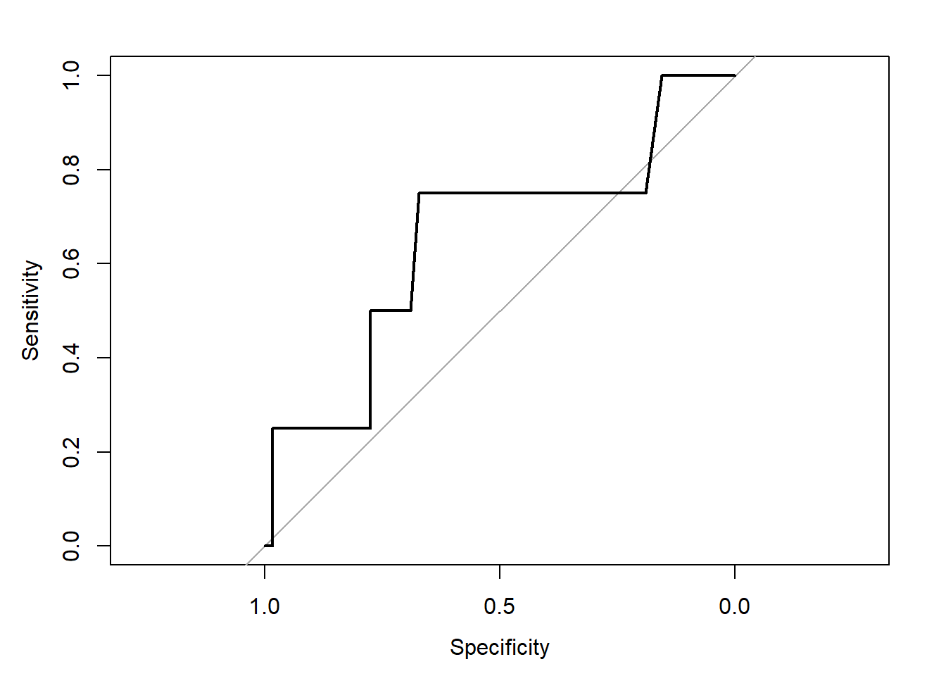

3c

Calculate the AUC, does it suggest any potential benefit?

Solution:

Code

roc3 # print the roc object output to extract the AUC

Call:
roc.formula(formula = SSI ~ VitaminD, data = dat3s)

Data: VitaminD in 58 controls (SSI 0) < 4 cases (SSI 1).
Area under the curve: 0.653

Code

auc(roc3) # specifically extract the AUC only

Area under the curve: 0.653

The AUC is estimated to be 0.653. Since this is greater than 0.5 it suggests vitamin D levels may be better than random chance (i.e., a coin flip), but is not necessarily a home run as far as biomarkers go (i.e., it isn’t a perfect predictor with AUC=1).

3d

The pROC package includes the ci.auc function that can calculate a confidence interval for your AUC. It does this in two ways, using either method=delong or method=bootstrap, where DeLong’s approach is based on asymptotics and the bootstrap is nonparametric. Calculate the 95% confidence interval for the AUC using either method. Based on this interval, if we are interested in testing \(H_0: AUC=0.5\) what would we conclude?

Solution:

Code

ci.auc(roc3)

95% CI: 0.3089-0.9971 (DeLong)

The 95% CI estimated with DeLong’s method is (0.3089, 0.9971). Since this includes the null value of 0.5, we cannot conclude that the vitamin D is a predictor that is better than random chance.

Note, in this problem we have both a small sample size after removing the NA values for vitamin D, but also only 4 patients with a surgical site infection. These smaller samples suggest we wouldn’t expect a very tight or narrow confidence interval in the first place.

Exercise 4: Sensitivity and Specificity

The following code can load the Licorice_Gargle.csv file into R:

Code

dat4 <- read.csv('../../.data/Licorice_Gargle.csv')

This was a randomized clinical trial of 236 adult patients undergoing elective thoracic surgery requiring a double-lumen endotracheal tube to compare if a licorice gargle prevents postoperative sore throat better than a sugar-water gargle.

The researchers are interested in seeing if BMI (preOp_calcBMI) can be used to predict who will report any pain at 30 minutes after surgery (pacu30min_throatPain is an 11-point Likert scale from 0=no pain to 10=worst pain).

4a

Subset the data to only include the control group (treat=0).

Solution:

Code

dat4s <- dat4[which(dat4$treat==0),]

4b

Create a 2x2 table summarizing an overweight BMI (i.e., BMI > 25) to predict any throat pain at 30 minutes (i.e., pain > 0).

Solution:

Code

tab4 <- table( overweight = factor(dat4s$preOp_calcBMI > 25, levels=c(T,F)), pain = factor(dat4s$pacu30min_throatPain > 0, levels=c(T,F))  )

tab4

          pain
overweight TRUE FALSE
     TRUE    24    44
     FALSE   18    30

4c

Calculate the sensitivity and specificity by hand from our 2x2 table and interpret.

Solution:

Sensitivity:

\(Se = P(T|D) = \frac{a}{a+c} = \frac{24}{24+18} = \frac{24}{42} = 0.571\)

Sensitivity Interpretation: If someone will have throat pain at 30 minutes, there is a 57.1% probability that their BMI > 25.

Specificity:

\(Sp = P(\bar{T}|\bar{D}) = \frac{d}{b+d} = \frac{30}{30+44} = \frac{30}{74} = 0.405\)

Specificity Interpretation: If someone will not have throat pain at 30 minutes, there is a 40.5% probability that their BMI < 25.

4d

Discuss if there is any potential use of BMI as a predictor of throat pain in those who are treated with a sugar-water placebo.

Solution:

Given the generally low sensitivity and specificity, there does not seem to be great potential utility of using BMI as a predictor for who will or will not have throat pain. In fact, these results suggest a false negative rate (\(FNR=1-Se\)) of 42.9% and a false positive rate (\(FPR=1-Sp\)) of 59.5%.