Week 11 Practice Problems: Solutions

Author

Affiliation

Alex Kaizer

University of Colorado-Anschutz Medical Campus

This page includes the solutions to the optional practice problems for the given week. If you want to see a version without solutions please click here. Data sets, if needed, are provided on the BIOS 6618 Canvas page for students registered for the course.

This week’s extra practice exercises focus on the wonderfully wide world of applications for MLR: confounding, mediation, interactions, general linear hypothesis testing, and polynomial regression.

Dataset Background

All of our exercises will use the surgery timing data set (Surgery_Timing.csv) provided by the TSHS section of the American Statistical Association. We can load the data into R with the following line of code:

Code

dat <- read.csv('../../.data/Surgery_Timing.csv')

The following table summarizes the variables we will be exploring and provide brief definitions:

Variable	Code Name	Description
Risk Stratification Index (RSI) for In-Hospital Complications	complication_rsi	Estimated risk of having an in-hospital complication.
Day of Week	dow	Weekday surgery took place (1=Monday, 5=Friday)
Operation Time	hour	Timing of operation during the day (06:00 to 19:00)
Phase of Moon	moonphase	Moon phase during procedure (1=new, 2=first quarter, 3=full, 4=last quarter)
Age	age	Age in years
BMI	bmi	Body mass index (kg/m2)
AHRQ Procedure Category	ahrq_ccs	US Agency for Healthcare Research and Quality’s Clinical Classifications Software procedure category
Complication Observed	complication	In-hospital complication
Diabetes	baseline_diabetes	Diabetes present at baseline

Exercise 1: Confounding

We will use linear regression to examine the relationship between the outcome of RSI for in-hospital complications with surgery on a Monday/Tuesday (versus Wednesday/Thursday/Friday) and moon phase to answer the following exercises:

1a: Unadjusted Model and Interpretation

What is the unadjusted (crude) estimate for the association between RSI and day of the week? Write a brief, but complete, summary of the relationship between RSI and day of the week. Hint: you will need to create a new variable for day of the week.

Solution:

Code

dat$AK_mt <- dat$dow %in% c(1,2)
mod1u <- lm(complication_rsi ~ AK_mt, data=dat)
summary(mod1u)

Call:
lm(formula = complication_rsi ~ AK_mt, data = dat)

Residuals:
    Min      1Q  Median      3Q     Max 
-4.3843 -0.4943  0.0757  0.4333 13.8033 

Coefficients:
             Estimate Std. Error t value Pr(>|t|)    
(Intercept) -0.335689   0.008956  -37.48   <2e-16 ***
AK_mtTRUE   -0.167634   0.013534  -12.39   <2e-16 ***
---
Signif. codes:  0 '***' 0.001 '**' 0.01 '*' 0.05 '.' 0.1 ' ' 1

Residual standard error: 1.201 on 31999 degrees of freedom
Multiple R-squared:  0.004772,  Adjusted R-squared:  0.004741 
F-statistic: 153.4 on 1 and 31999 DF,  p-value: < 2.2e-16

Code

confint(mod1u)

                 2.5 %     97.5 %
(Intercept) -0.3532430 -0.3181357
AK_mtTRUE   -0.1941607 -0.1411073

There is a significant relationship between RSI for in-hospital complications and day of week (M/T vs. W/Th/F) (p<0.001). On average, RSI is 0.17 lower (95% CI: 0.14 to 0.19 lower) on M/T compared to W/Th/F surgeries.

1b: Adjusted Model and Interpretation

Adjusting for the effect of moon phase, what is the adjusted estimate for the association between RSI and day of the week? Write a brief, but complete, summary of the relationship between RSI and day of the week adjusting for moon phase.

Solution:

Code

mod1a <- lm(complication_rsi ~ AK_mt + as.factor(moonphase), data=dat)
summary(mod1a)

Call:
lm(formula = complication_rsi ~ AK_mt + as.factor(moonphase), 
    data = dat)

Residuals:
    Min      1Q  Median      3Q     Max 
-4.3828 -0.4928  0.0772  0.4278 13.8247 

Coefficients:
                      Estimate Std. Error t value Pr(>|t|)    
(Intercept)           -0.32039    0.01490 -21.507   <2e-16 ***
AK_mtTRUE             -0.16740    0.01354 -12.369   <2e-16 ***
as.factor(moonphase)2 -0.03689    0.01911  -1.930   0.0536 .  
as.factor(moonphase)3 -0.00707    0.01914  -0.369   0.7118    
as.factor(moonphase)4 -0.01682    0.01909  -0.881   0.3782    
---
Signif. codes:  0 '***' 0.001 '**' 0.01 '*' 0.05 '.' 0.1 ' ' 1

Residual standard error: 1.201 on 31996 degrees of freedom
Multiple R-squared:  0.004904,  Adjusted R-squared:  0.00478 
F-statistic: 39.42 on 4 and 31996 DF,  p-value: < 2.2e-16

Code

confint(mod1a)

                            2.5 %        97.5 %
(Intercept)           -0.34959437 -0.2911952782
AK_mtTRUE             -0.19393341 -0.1408770162
as.factor(moonphase)2 -0.07434743  0.0005763537
as.factor(moonphase)3 -0.04458653  0.0304459049
as.factor(moonphase)4 -0.05423393  0.0205935279

There is a significant relationship between RSI for in-hospital complications and day of week (M/T vs. W/Th/F) (p<0.001). After accounting for moon phase, on average, RSI is 0.17 lower (95% CI: 0.14 to 0.19 lower) on M/T compared to W/Th/F surgeries.

1c: Moon Phase Confounding

Is moon phase a confounder of the association between RSI and day of the week based on the operational criterion? Should you report the results from (A) or (B)? Justify your answer.

Solution:

Moon phase is not a confounder by the operational definition, since it does not greatly change our point estimate of M/T vs. W/Th/F:

\[ \frac{|0.167634 - 0.16740|}{0.167634} \times 100 = 0.1396% \]

While there is no rigid threshold for a change that is “big” enough, this is rather small and <10% or <20% are commonly used to rule out potential confounding with the operational definition.

Exercise 2: Mediation

We will use linear regression to examine the relationship between the outcome of RSI for in-hospital complications with surgery on a Monday/Tuesday (versus Wednesday/Thursday/Friday) and BMI of the patient potential mediator to complete the following exercises:

2a: Mediation DAG

Fit the three fundamental models of mediation analysis and fill in the following DAG:

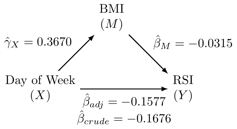
Solution:

Code

# Fit our three models
mod2_crude <- lm(complication_rsi ~ AK_mt, data=dat)
mod2_adjusted <- lm(complication_rsi ~ AK_mt + bmi, data=dat)
mod2_covariate <- lm(bmi ~ AK_mt, data=dat)

# Extract coefficients
coef(mod2_crude)

(Intercept)   AK_mtTRUE 
 -0.3356893  -0.1676340 

Code

coef(mod2_adjusted)

(Intercept)   AK_mtTRUE         bmi 
 0.57313211 -0.15765353 -0.03148069 

Code

coef(mod2_covariate)

(Intercept)   AK_mtTRUE 
  29.290095    0.367003 

2b: Percent Mediated

What is the proportion/percent mediated by age?

Solution:

The proportion mediated is \(\frac{\text{indirect effect}}{\text{total effect}} = \frac{\hat{\beta}_{crude} - \hat{\beta}_{adj}}{\hat{\beta}_{crude}} = \frac{-0.1676 - (-0.1577)}{-0.1676} = 0.0591\). This corresponds to the percent mediated of \(0.0591 \times 100 = 5.91\%\).

2c: 95% CI for Percent Mediated

What is the 95% CI and corresponding p-value for the proportion/percent mediated by age using the normal approximation to estimate the standard error (i.e., Sobel’s test)?

Solution:

We first need to calculate the standard error for our indirect effect:

\[ SE(\hat{\beta}_{crude} - \hat{\beta}_{adj}) = \sqrt{{\hat{\gamma}}_X^2\left(SE\left({\hat{\beta}}_M\right)\right)^2+{\hat{\beta}}_M^2\left(SE\left({\hat{\gamma}}_X\right)\right)^2} \]

We can find this information in our coefficient tables:

Code

summary(mod2_adjusted)$coefficient

               Estimate   Std. Error   t value      Pr(>|t|)
(Intercept)  0.57313211 0.0290929009  19.70007  7.953691e-86
AK_mtTRUE   -0.15765353 0.0138026533 -11.42197  3.773477e-30
bmi         -0.03148069 0.0009427987 -33.39068 7.305638e-240

Code

summary(mod2_covariate)$coefficient

             Estimate Std. Error    t value     Pr(>|t|)
(Intercept) 29.290095 0.05731452 511.041478 0.000000e+00
AK_mtTRUE    0.367003 0.08637699   4.248851 2.155467e-05

\[ SE(\hat{\beta}_{crude} - \hat{\beta}_{adj}) = \sqrt{(0.3670)^2(0.0009)^2 + (-0.0315)^2 (0.0864)^2} = 0.0027 \]

Our 95% CI for the indirect effect is

\[ (-0.1676 - (-0.1577)) \pm 1.96 \times 0.0027 = (-0.015, -0.005) \]

This corresponds to a 95% CI for our proportion mediated of:

\[ \left(\frac{-0.005}{-0.1676}, \frac{-0.015}{-0.1676} \right) = (0.0298, 0.0895)) \]

We are 95% confident that the proportion mediated by BMI is betwee 2.98% and 8.95%.

Our p-value is calculated from referencing the standard normal distribution (per Sobel’s test):

\[ Z = \frac{\text{indirect effect}}{SE(\hat{\beta}_{crude} - \hat{\beta}_{adj})} = \frac{-0.0099}{0.0027} = -3.67 \]

This corresponds to a p-value of 2 * pnorm(-3.67)=2.4^{-4}, which is less than 0.05.

Note, that although this proportion mediated is not very large, our larger sample size may be powered enough to detect even weak mediation relationships.

Exercise 3: Interactions

Use linear regression to examine the relationship between RSI for in-hospital complications and BMI. In this exercise you will examine whether the magnitude of the association between RSI (the response) and BMI (the primary explanatory variable) depends on whether the patient has diabetes.

3a: Fitted Regression Equation with Interaction

Write down the fitted regression equation for the regression of RSI on BMI, diabetes, and the interaction between the two. Provide an interpretation for each of the coefficients in the model (including the intercept).

Solution:

Code

mod3 <- lm( complication_rsi ~ bmi + baseline_diabetes + bmi*baseline_diabetes, data=dat)

cbind(summary(mod3)$coef, confint(mod3))

                         Estimate  Std. Error    t value      Pr(>|t|)
(Intercept)            0.53713273 0.031985132  16.793200  5.472708e-63
bmi                   -0.03156706 0.001080522 -29.214640 6.452865e-185
baseline_diabetes     -0.64875563 0.082053863  -7.906461  2.742595e-15
bmi:baseline_diabetes  0.01223915 0.002424084   5.048979  4.468924e-07
                             2.5 %      97.5 %
(Intercept)            0.474440377  0.59982508
bmi                   -0.033684938 -0.02944919
baseline_diabetes     -0.809585030 -0.48792624
bmi:baseline_diabetes  0.007487831  0.01699046

Our fitted regression model is

\[ \hat{Y} = 0.537 + -0.032 \times \text{BMI} + -0.649 \times \text{diabetes} + 0.012 \times \text{BMI} \times \text{diabetes} \]

\(\hat{\beta}_0 = 0.537\): The expected RSI for patients with a 0 kg/m² BMI and who do not have diabetes is 0.537 points.

\(\hat{\beta}_{bmi}=-0.032\): For patients who do not have diabetes, RSI decreases, on average, by 0.032 points for 1 kg/m² increase in BMI.

\(\hat{\beta}_{diabetes}=-0.649\): For patients with a 0 kg/m² BMI, RSI, on average, is 0.649 points lower for those with diabetes.

\(\hat{\beta}_{bmi*diabetes} = 0.012\): This is the difference between the effect of BMI for those with diabetes compared to those without diabetes. For patients with diabetes, a one kg/m² increase in BMI results in an RSI that is 0.012 units higher, on average.

3b: Interaction Test

Test whether the relationship between RSI and BMI depends on whether the patient had diabetes.

Solution:

From our model results in 3a, the relationship between RSI and BMI is significantly different for those with diabetes compared to those without diabetes (p=4.47e-07<0.001).

3c: Fitted Regression Model for Patients without Diabetes

What is the regression equation for patients who don’t have diabetes?

Solution:

\[ \hat{Y} = 0.537 + -0.032 \times \text{BMI} + -0.649 \times 0 + 0.012 \times \text{BMI} \times 0 = 0.537 + -0.032 \times \text{BMI} \]

3d: Fitted Regression Model for Patients with Diabetes

What is the regression equation for patients with diabetes?

Solution:

\[ \hat{Y} = 0.537 + -0.032 \times \text{BMI} + -0.649 \times 1 + 0.012 \times \text{BMI} \times 1 = -0.112 + -0.020 \times \text{BMI} \]

3e: Interaction Visualization

Create a scatterplot of RSI versus BMI, using different symbols and separate regression lines for patients with and without diabetes.

Solution:

Code

plot(x=dat$bmi, y=dat$complication_rsi, xlab='BMI', ylab='RSI', pch=dat$baseline_diabetes)
abline(a=0.537, b=-0.032, lty=1, col='orangered2')
abline(a=-0.112, b=-0.020, lty=2, col='orangered2')
legend('topright', bty='n', pch=c(0,1), lty=c(1,2),
       legend=c('No Diabetes','Diabetes'))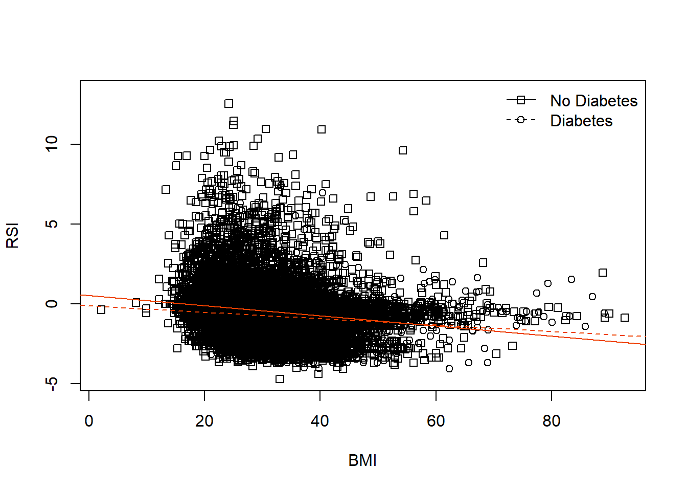

3f: Hypothesis Test for BMI without Diabetes

Test if the slope for BMI for those who don’t have diabetes is significantly different from 0.

Solution:

For this question we can directly use the \(t\)-test results from our table of coefficients in 3A. In that output we see that p<2e-16 for bmi, so we reject the null hypothesis that the slope is significantly different from 0 for those who didn’t have diabetes.

3g: Hypothesis Test for BMI with Diabetes

Test if the slope for BMI for those who do have diabetes is significantly different from 0.

Solution:

For this question we can approach it by either calculating the standard error of \(\hat{\beta}_{bmi} + \hat{\beta}_{bmi*diabetes}\) or using reverse coding.

Calculating the standard error using our original model requires the variance-covariance matrix:

Code

vcov(mod3)

                        (Intercept)           bmi baseline_diabetes
(Intercept)            1.023049e-03 -3.363775e-05     -1.023049e-03
bmi                   -3.363775e-05  1.167528e-06      3.363775e-05
baseline_diabetes     -1.023049e-03  3.363775e-05      6.732836e-03
bmi:baseline_diabetes  3.363775e-05 -1.167528e-06     -1.923745e-04
                      bmi:baseline_diabetes
(Intercept)                    3.363775e-05
bmi                           -1.167528e-06
baseline_diabetes             -1.923745e-04
bmi:baseline_diabetes          5.876182e-06

With this information we can calculate our standard error:

\(\begin{aligned} SE(\hat{\beta}_{bmi} + \hat{\beta}_{bmi*diabetes}) =& \sqrt{Var(\hat{\beta}_{bmi}) + Var(\hat{\beta}_{bmi*diabetes}) + 2 \times Cov(\hat{\beta}_{bmi},\hat{\beta}_{bmi*diabetes})} \\ =& \sqrt{1.167528e-06 + 5.876182e-06 + 2 \times (-1.167528e-06)} \\ =& \sqrt{4.708654e-06} \\ =& 0.002169943 \end{aligned}\)

Our estimated 95% CI using a critical value of 1.96 (i.e., qt(0.975, 28707) based on \(n=28711\) with complete data for BMI and diabetes status and subtracting four degrees of freedom) is

\[ -0.020 \pm 1.96 \times 0.002169943 = (-0.0243, -0.0157) \]

We have \(t=\frac{-0.020}{0.002169943}=-9.217\) and a p-value of 2 * pt(-9.217,28707,lower.tail=T)=0.

We can verify this result if we reverse code baseline_diabetes:

Code

# create reverse coding where not_first2y=1 if they did NOT live in first 2 years
dat$AK_no_diabetes <- abs(dat$baseline_diabetes - 1)

# fit model with reverse coding
mod3_reverse <- lm(complication_rsi ~ bmi + AK_no_diabetes + bmi*AK_no_diabetes, data=dat)
round( cbind(summary(mod3_reverse)$coefficients, confint(mod3_reverse)), 4)

                   Estimate Std. Error t value Pr(>|t|)   2.5 %  97.5 %
(Intercept)         -0.1116     0.0756 -1.4772   0.1396 -0.2597  0.0365
bmi                 -0.0193     0.0022 -8.9071   0.0000 -0.0236 -0.0151
AK_no_diabetes       0.6488     0.0821  7.9065   0.0000  0.4879  0.8096
bmi:AK_no_diabetes  -0.0122     0.0024 -5.0490   0.0000 -0.0170 -0.0075

We can see that we arrive at the same results (with slight differences due to rounding) when interpreting bmi in our reverse coded model results.

3h: Interactions and Brief, but Complete, Summaries

Provide a brief, but complete, summary of the relationship between RSI and BMI, accounting for any observed interaction with diabetes (i.e., if there is a significant interaction, interpret those who do and don’t have diabetes separately).

Solution:

The relationship between BMI and RSI differs significantly according to whether or not the patient has diabetes (p<0.001).

There is a significant association between BMI and RSI for patients without diabetes (p < 0.001). For these patients, RSI decreases an average of 0.032 units for every one kg/m² increase in BMI (95% CI: 0.0294 to 0.0337 units lower).

There is a significant association between BMI and RSI among patients with diabetes (p < 0.001). For these patients, RSI decreases an average of 0.020 units for every one kg/m² increase in BMI (95% CI: 0.0157 to 0.0243 units lower).

The difference in these relationships for patients with and without diabetes can be seen in the scatterplot with regression fits for each group, where those without diabetes have a slightly stronger negative linear relationship with RSI as BMI increases.

Exercise 4: Polynomial Regression

For this exercise, subset the data set to only those with an in-hospital complication recorded and those who have hip replacements (i.e., dat$ahrq_ccs=='Hip replacement; total and partial').

4a: SLR

Fit a simple linear regression model for the outcome of RSI for in-hospital complications with age as the predictor.

Solution:

Code

dat4 <- dat[which(dat$complication==1 & dat$ahrq_ccs=='Hip replacement; total and partial'),]

dat4 <- dat4[!is.na(dat4$age),] # remove one record without age

lm4 <- lm(complication_rsi ~ age, data=dat4)

4b: Polynomial Regression

Fit a polynomial regression model that adds a squared term for age.

Solution:

Code

lm4_2 <- lm(complication_rsi ~ age + I(age^2), data=dat4)

4c: Polynomial Plots

Create a scatterplot of the data and add the predicted regression lines for each model.

Solution:

Code

plot(x=dat4$age, y=dat4$complication_rsi, xlab='Age', ylab='RSI (In-Hospital Complications)')
abline(lm4, lwd=2) # plot SLR predicted regression line

# predict Y-hat from regression model with age and age^2, add to scatterplot
xval <- seq(min(dat4$age,na.rm=T), max(dat4$age,na.rm=T), length.out=100)
y2 <- predict(lm4_2, newdata = data.frame(age=xval))
lines(x=xval, y=y2, col='blue', lwd=2, lty=2)

# add legend
legend('topleft', bty='n', col=c('black','blue'), lwd=c(2,2), lty=c(1,2), legend=c('Linear','Quadratic'))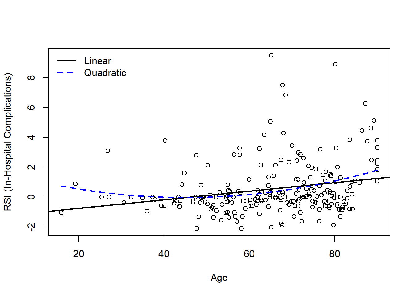

4d: Polynomial vs SLR

Based on the model output and figure, is there evidence that a quadratic model may be more appropriate than the simple linear regression model?

Solution:

Visually, both models may be appropriate. There are fewer young patients, so it can be challenging to definitely identify if the linear or quadratic model is more appropriate. While we know that age and age² are highly correlated, we can examine our summary output to note that age² is significant in the quadratic model (p<0.05):

Code

summary(lm4)

Call:
lm(formula = complication_rsi ~ age, data = dat4)

Residuals:
    Min      1Q  Median      3Q     Max 
-2.8344 -1.0164 -0.4061  0.5047  8.9619 

Coefficients:
             Estimate Std. Error t value Pr(>|t|)    
(Intercept) -1.307892   0.535371  -2.443 0.015352 *  
age          0.028510   0.007953   3.585 0.000415 ***
---
Signif. codes:  0 '***' 0.001 '**' 0.01 '*' 0.05 '.' 0.1 ' ' 1

Residual standard error: 1.772 on 221 degrees of freedom
Multiple R-squared:  0.05495,   Adjusted R-squared:  0.05067 
F-statistic: 12.85 on 1 and 221 DF,  p-value: 0.0004152

Code

summary(lm4_2)

Call:
lm(formula = complication_rsi ~ age + I(age^2), data = dat4)

Residuals:
    Min      1Q  Median      3Q     Max 
-2.9407 -0.9988 -0.3736  0.4102  9.1707 

Coefficients:
              Estimate Std. Error t value Pr(>|t|)  
(Intercept)  1.8377058  1.4762057   1.245   0.2145  
age         -0.0827367  0.0493547  -1.676   0.0951 .
I(age^2)     0.0009173  0.0004018   2.283   0.0234 *
---
Signif. codes:  0 '***' 0.001 '**' 0.01 '*' 0.05 '.' 0.1 ' ' 1

Residual standard error: 1.755 on 220 degrees of freedom
Multiple R-squared:  0.07683,   Adjusted R-squared:  0.06843 
F-statistic: 9.154 on 2 and 220 DF,  p-value: 0.0001517

We can also calculate the MSE to see if it decreases in the quadratic model relative to the first-order model without any polynomial terms:

Code

mean(lm4$residuals^2) # MSE for first-order model

[1] 3.110576

Code

mean(lm4_2$residuals^2) # MSE for second-order model

[1] 3.038569

Since the change in MSE is not very large (3.11 to 3.04), we might argue the more parsimonious SLR model may be preferred given the limited improvement relative to the increased complexity.

Finally, we may want to evalute the diagnostic plots to see if there is evidence to support the more complex model:

Code

# SLR diagnostics (no quadratic term)
par(mfrow=c(2,3), mar=c(4.1,4.1,3.1,2.1))

# Scatterplot of Y-X
plot(x=dat4$age, y=dat4$complication_rsi, xlab='Age', ylab='RSI', 
     main='Scatterplot', cex=1); abline( lm4, col='blue', lwd=2 )

# Scatterplot of residuals by X
plot(x=dat4$age, y=rstudent(lm4), xlab='Age', ylab='Jackknife Residual', 
     main='Residual Plot by Age', cex=1); abline(h=0, lty=2, col='gray65')

# Scatterplot of residuals by predicted values
plot(x=predict(lm4), y=rstudent(lm4), xlab=expression(hat(Y)), ylab='Jackknife Residual', 
     main='Residual Plot by Y-hat', cex=1); abline(h=0, lty=2, col='gray65')

# Histogram of jackknife residuals with normal curve
hist(rstudent(lm4), xlab='Jackknife Residual', 
     main='Histogram of Residuals', freq=F, breaks=seq(-5,6,0.25)); 
  curve( dnorm(x,mean=0,sd=1), lwd=2, col='blue', add=T)

# PP-plot
plot( ppoints(length(rstudent(lm4))), sort(pnorm(rstudent(lm4))), 
      xlab='Observed Cumulative Probability', 
      ylab='Expected Cumulative Probability', 
      main='Normal Probability Plot', cex=1); 
  abline(a=0,b=1, col='gray65', lwd=1)

# QQ-plot
qqnorm( rstudent(lm4) ); qqline( rstudent(lm4) )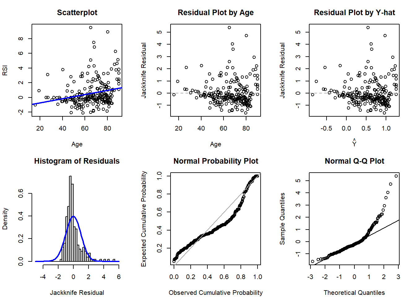

Code

# SLR diagnostics (no quadratic term)
par(mfrow=c(2,3), mar=c(4.1,4.1,3.1,2.1))

# Scatterplot of Y-X
plot(x=dat4$age, y=dat4$complication_rsi, xlab='Age', ylab='RSI', 
     main='Scatterplot', cex=1)
# predict Y-hat from regression model with age and age^2, add to scatterplot
xval <- seq(min(dat4$age,na.rm=T), max(dat4$age,na.rm=T), length.out=100)
y2 <- predict(lm4_2, newdata = data.frame(age=xval))
lines(x=xval, y=y2, col='blue', lwd=2)

# Scatterplot of residuals by X
plot(x=dat4$age, y=rstudent(lm4_2), xlab='Age', ylab='Jackknife Residual', 
     main='Residual Plot by Age', cex=1); abline(h=0, lty=2, col='gray65')

# Scatterplot of residuals by predicted values
plot(x=predict(lm4_2), y=rstudent(lm4_2), xlab=expression(hat(Y)), ylab='Jackknife Residual', 
     main='Residual Plot by Y-hat', cex=1); abline(h=0, lty=2, col='gray65')

# Histogram of jackknife residuals with normal curve
hist(rstudent(lm4_2), xlab='Jackknife Residual', 
     main='Histogram of Residuals', freq=F, breaks=seq(-5,6,0.25)); 
  curve( dnorm(x,mean=0,sd=1), lwd=2, col='blue', add=T)

# PP-plot
plot( ppoints(length(rstudent(lm4_2))), sort(pnorm(rstudent(lm4_2))), 
      xlab='Observed Cumulative Probability', 
      ylab='Expected Cumulative Probability', 
      main='Normal Probability Plot', cex=1); 
  abline(a=0,b=1, col='gray65', lwd=1)

# QQ-plot
qqnorm( rstudent(lm4_2) ); qqline( rstudent(lm4_2) )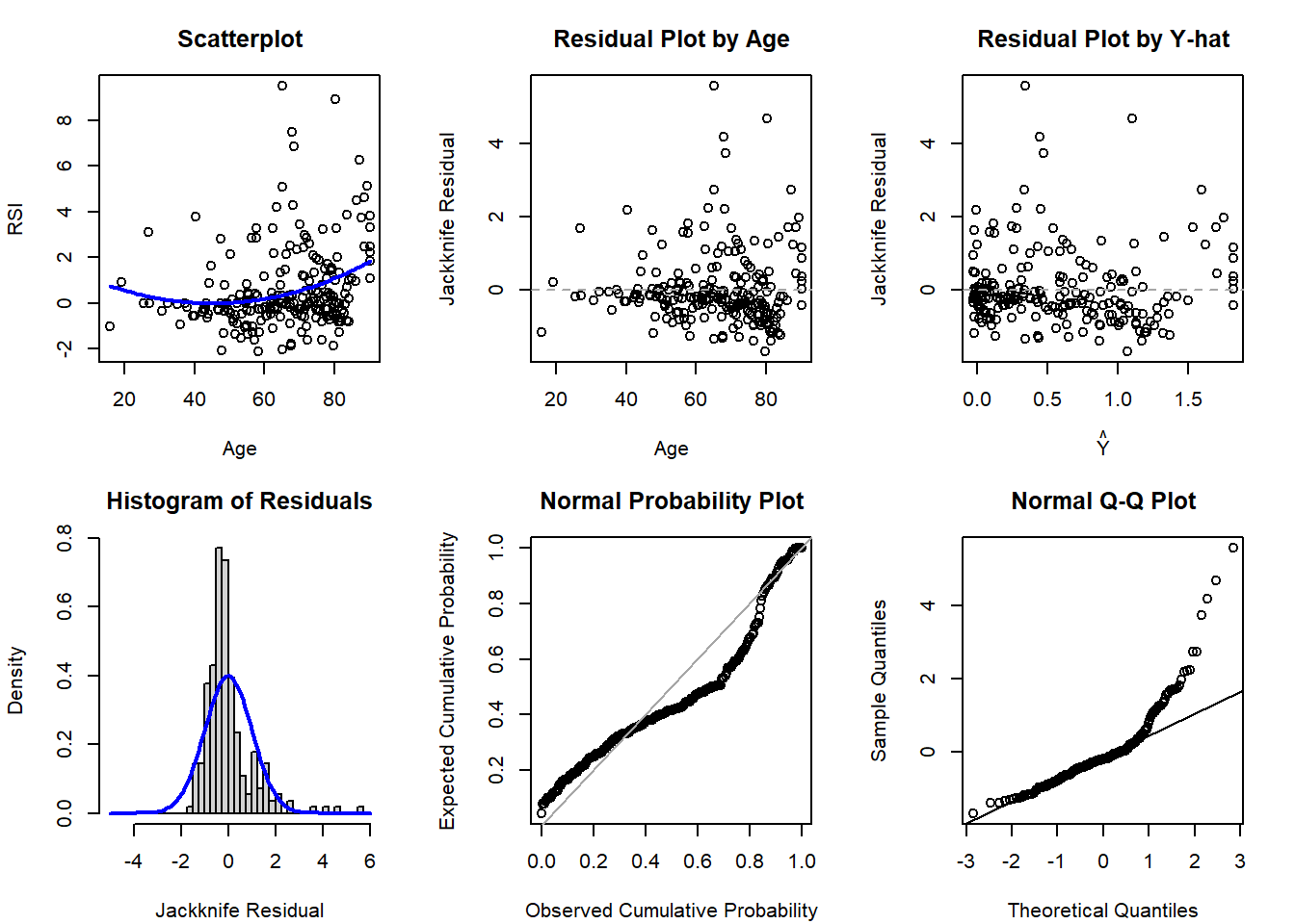

Based on the diagnostic plots, it appears both models are impacted by violations of the normality (histogram, PP, and QQ plots all have departures from normality) and potentially homoscedasticity assumption (residual plot by age might have a bit of a fan shape, but Y-hat not as much). Regardless, if just comparing to select between the first- and second-order model, there is not much evidence supporting a drastic improvement with the more complicated model with the quadratic polynomial term.

Exercise 5: Tests of General Linear Hypotheses

5a: Fitting The Model

Fit a linear regression model for the outcome of RSI for in-hospital complication with day of the week as a predictor for all days.

Solution:

Here we will fit our model and view the summary output for use in later problems.

Code

mod5 <- glm(complication_rsi ~ as.factor(dow), data=dat)
summary(mod5)

Call:
glm(formula = complication_rsi ~ as.factor(dow), data = dat)

Coefficients:
                Estimate Std. Error t value Pr(>|t|)    
(Intercept)     -0.51529    0.01435 -35.907  < 2e-16 ***
as.factor(dow)2  0.02393    0.02029   1.179    0.238    
as.factor(dow)3  0.18989    0.02088   9.092  < 2e-16 ***
as.factor(dow)4  0.15168    0.02149   7.057 1.73e-12 ***
as.factor(dow)5  0.19485    0.02105   9.258  < 2e-16 ***
---
Signif. codes:  0 '***' 0.001 '**' 0.01 '*' 0.05 '.' 0.1 ' ' 1

(Dispersion parameter for gaussian family taken to be 1.442609)

    Null deviance: 46388  on 32000  degrees of freedom
Residual deviance: 46158  on 31996  degrees of freedom
AIC: 102549

Number of Fisher Scoring iterations: 2

Our fitted regression equation is

\[\hat{Y} = -0.52 + 0.02 I_{T} + 0.19 I_{W} + 0.15 I_{Th} + 0.19 I_{F} \]

5b: GLHT for Two Coefficients

Using a general linear hypothesis, test if the mean RSI on Tuesday and Wednesday are equal to each other.

Solution:

First, if we want to compare the mean RSI value for each day we know from our reference cell model we would have an estimate of the mean for each group as \(\mu_{T} = \beta_0 + \beta_T\) and \(\mu_{W} = \beta_0 + \beta_{W}\). However, since our intercept \(\beta_0\) is in both, it will cancel out when testing our null hypothesis that \(\mu_T = \mu_W\).

Therefore, this tests \(H_0\colon \beta_{T} = \beta_{W}\), or equivalently \(H_0\colon \beta_{T} - \beta_{W} = 0\). We can further imagine this as \(1 \times \beta_{T} - 1 \times \beta_{W}\), so our matrix is \(\mathbf{c} = \begin{pmatrix} 0 & 1 & -1 & 0 & 0 \end{pmatrix}\):

Code

library(gmodels)

Warning: package 'gmodels' was built under R version 4.4.1

Code

# First, create matrix for given contrast
c_matrix_5b <- rbind( c(0,1,-1,0,0) )

# Then, implement general linear hypothesis test
glh.test(mod5, c_matrix_5b, d=rep(0,nrow(c_matrix_5b)))

     Test of General Linear Hypothesis  
Call:
glh.test(reg = mod5, cm = c_matrix_5b, d = rep(0, nrow(c_matrix_5b)))
F = 63.1627, df1 =     1, df2 = 31996, p-value = 1.998e-15 

Since \(p<0.05\), we would reject the null hypothesis and conclude that Tuesday and Wednesday have different mean RSI values.

Since we only wanted to compare if Tuesday and Wednesday were equal, we could also have fit a model with the reference category for our categorical variable changed to Tuesday or Wednesday:

Code

dat$dow_v2 <- factor(dat$dow, levels=c(2,3,4,5,1), labels=c('T','W','Th','F','M'))
summary( glm(complication_rsi ~ dow_v2, data=dat))

Call:
glm(formula = complication_rsi ~ dow_v2, data = dat)

Coefficients:
            Estimate Std. Error t value Pr(>|t|)    
(Intercept) -0.49136    0.01435 -34.247  < 2e-16 ***
dow_v2W      0.16596    0.02088   7.947 1.97e-15 ***
dow_v2Th     0.12775    0.02149   5.945 2.80e-09 ***
dow_v2F      0.17093    0.02104   8.122 4.74e-16 ***
dow_v2M     -0.02393    0.02029  -1.179    0.238    
---
Signif. codes:  0 '***' 0.001 '**' 0.01 '*' 0.05 '.' 0.1 ' ' 1

(Dispersion parameter for gaussian family taken to be 1.442609)

    Null deviance: 46388  on 32000  degrees of freedom
Residual deviance: 46158  on 31996  degrees of freedom
AIC: 102549

Number of Fisher Scoring iterations: 2

In our regression output with Tuesday as the reference category, we see we have a similar p-value and that \(t^2 = 7.946^2 = 63.139\), which is approximately equal to our \(F\)-statistic from the GLHT (differing slightly due to rounding).

5c: GLHT for Combination of Coefficients

Using a general linear hypothesis, test if the mean RSI on Monday is equal to two times the RSI on Thursday.

Solution:

Here we know that for our model fit in 5a, \(\mu_M = \beta_0\) and \(\mu_{Th} = \beta_0 + \beta_{Th}\). Therefore this hypothesis is testing the null that \(\mu_M = 2 \times \mu_{Th}\). Plugging in our regression coefficients we have \(\beta_0 = 2 \times (\beta_0 + \beta_{Th})\). This can be rearranged to show that \(-\beta_0 + 2\beta_{Th} = 0\):

\[ H_0 \colon \begin{pmatrix} -1 & 0 & 0 & 2 & 0 \end{pmatrix} \begin{pmatrix} \beta_0 \\ \beta_T \\ \beta_W \\ \beta_{Th} \\ \beta_{F} \end{pmatrix} = 0 \]

Code

# First, create matrix for given contrast
c_matrix_5c <- rbind( c(-1,0,0,2,0) )

# Then, implement general linear hypothesis test
glh.test(mod5, c_matrix_5c, d=rep(0,nrow(c_matrix_5c)))

     Test of General Linear Hypothesis  
Call:
glh.test(reg = mod5, cm = c_matrix_5c, d = rep(0, nrow(c_matrix_5c)))
F = 232.9077, df1 =     1, df2 = 31996, p-value = < 2.2e-16 

Since \(p < 0.05\), we reject \(H_0\) and conclude that the mean RSI on Monday is not equal to two times the mean RSI on Thursday.

5d: GLHT for Simultaneous Testing

Using a general linear hypothesis, test both 5b and 5c simultaneously.

Solution:

For 5b and 5c, we tested each hypothesis on its own. However, we could test both simultaneously:

\[ H_0 \colon \begin{pmatrix} 0 & 1 & -1 & 0 & 0 \\ -1 & 0 & 0 & 2 & 0 \end{pmatrix} \begin{pmatrix} \beta_0 \\ \beta_T \\ \beta_W \\ \beta_{Th} \\ \beta_{F} \end{pmatrix} = \begin{pmatrix} 0 \\ 0 \end{pmatrix} \]

Code

# First, create matrix for given contrast
c_matrix_5d <- rbind( c(0,1,-1,0,0), c(-1,0,0,2,0) )

# Then, implement general linear hypothesis test
glh.test(mod5, c_matrix_5d, d=rep(0,nrow(c_matrix_5d)))

     Test of General Linear Hypothesis  
Call:
glh.test(reg = mod5, cm = c_matrix_5d, d = rep(0, nrow(c_matrix_5d)))
F = 148.0352, df1 =     2, df2 = 31996, p-value = < 2.2e-16 

Unsurprisingly, given our previous results with both being very significant on their own, this result is still also significant since \(p<0.001\). In other words, our results suggests that at least one null hypothesis is rejected.