This page is part of the University of Colorado-Anschutz Medical Campus’ BIOS 6618 Recitation collection. To view other questions, you can view the BIOS 6618 Recitation collection page or use the search bar to look for keywords.
Wilcoxon Rank Sum Examples
Homework 5, Question 4c
Let’s see how we can compare our length of stay data for HW 5, Question 4c, by implementing the WRS “by-hand” before checking our answers with a function in R.
Since we have \(n_{\text{Cauchy}} = 12 \ge 10\) and \(n_{\text{Skellam}} = 15 \ge 10\), we can use the asymptotic approach. Here, we will use the Cauchy General Hospital as our group for the calculations.
First, we can sum up the average ranks corresponding to our Cauchy LOS data: [ R_{} = 1.5+1.5+3+5+5+5+7.5+11+11+15.5+19+26.5 = 111.5 ]
Then, we can calculate our expected value for \(R_{\text{Cauchy}}\): [ E= = = = 168 ].
Finally, we can calculate the variance for our statistic (recall, \(g\) is values with ties and \(t_i\) is the number of ties at a given value):
    Asymptotic Wilcoxon-Mann-Whitney Test

data:  los by cauchy (0, 1)
Z = 2.7752, p-value = 0.005517
alternative hypothesis: true mu is not equal to 0
We see we are pretty close to the function output (with differences likely due to rounding in our “by-hand” calculations).
Exact Version of Wilcoxon Rank Sum
If our sample sizes are too small (e.g., either <10 based on our lecture slides), it may be more appropriate to use an exact approach instead of the normal approximation.
In our case, the normal approximation would be considered acceptable. However, for illustration purpose let’s assume from our nonparametric lecture slide 8/27, we have \(n_1=9\) and \(n_2=10\) (i.e., Table 12 from the Rosner textbook).
In this case, for \(\alpha=0.05\), we have \(T_{l}-T_{r} = 65-115\). For \(T=R_1=415.3846\) we would note that \(415.3846 = T > T_r = 115\). Then, we’d conclude from our table reference that we reject \(H_0\) and there is a difference in the mean ranks between our two groups.
The WRS In Practice
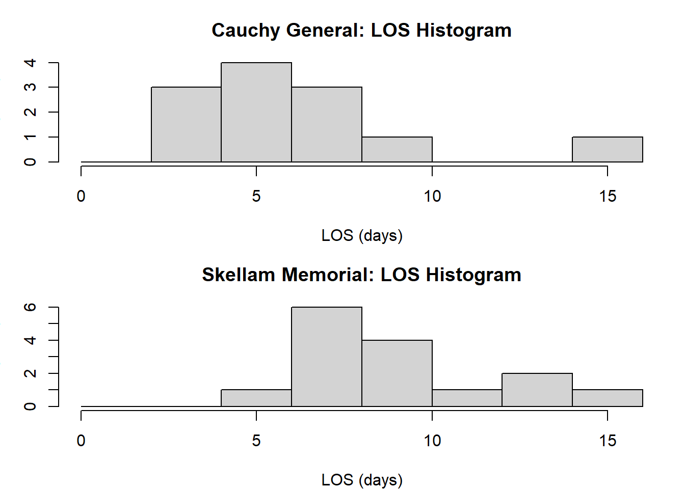
We’ve noted many, many times that the WRS is NOT a test of the medians unless we make the somewhat strong assumption that the shapes of the distributions are identical (i.e., only the “location” of the median is changing). In practice, we often evaluate this graphically by making histograms or boxplots of our data:
The big challenge is that with smaller samples, it can be really hard to determine if the shapes are really identical. If we are able or willing to get more data, we might be able to more confidently decide if the shapes are identical enough to meet the assumption. However, you may also be veering into sample sizes where the central limit theorem kicks in for the t-test (i.e., even if the underlying data isn’t normal, we know that the sample means are normally distributed with large enough sample sizes). Alternatively, we can use other tests (e.g., Mood’s test of the median between two independent samples, quantile regression) that are already testing the median.
Creating Data Frames with Vectorized Data
When using some functions, we have flexibility to provide vectors, matrices, and/or data frames for data elements. In certain cases, a function may require a specific formatting of the data. For example, coin::wilcox_test() expects data in the form of a formulaic representation (i.e., likely using a data frame for the data).
Fortunately, for our homework problem the data is relatively short and we can manually create a data frame in a few ways.
Approach 1/1b creates a single data frame by replicating the site (Cauchy=1/Skellam=0 as a factor meet the wilcox_test expected type of data) and copying the vector of values directly or as objects:
Code
# Approach 1 (Alex's preferred): combine the data in one DFdf1 <-data.frame(cauchy=factor(c(rep(1,12), rep(0,15))), los=c(3, 3, 4, 5, 5, 5, 6, 7, 7, 8, 9, 15,6, 7, 7, 7, 8, 8, 8, 9, 9, 10, 10, 11, 13, 13, 15))df1[c(1:3,25:27),]
Approach 2 creates two separate data frames and then merges them together (but we need to be careful they have the same column names!):
Code
# Approach 2: create two separate data frames and mergenew <-data.frame(cauchy=factor(1), los = new)soc <-data.frame(cauchy=factor(0),los = soc)df2 <-rbind( new, soc) # use rbind to merge two objects with same column namesdf2[c(1:3,25:27),]
class(df2$cauchy) # check data type is still factor
[1] "factor"
Source Code
---title: "Wilcoxon Rank Sum Examples and Using Vectorized Data in Functions"author: name: Alex Kaizer roles: "Instructor" affiliation: University of Colorado-Anschutz Medical Campustoc: truetoc_float: truetoc-location: leftformat: html: code-fold: show code-overflow: wrap code-tools: true---```{r, echo=F, message=F, warning=F}library(kableExtra)library(dplyr)```This page is part of the University of Colorado-Anschutz Medical Campus' [BIOS 6618 Recitation](/recitation/index.qmd) collection. To view other questions, you can view the [BIOS 6618 Recitation](/recitation/index.qmd) collection page or use the search bar to look for keywords.# Wilcoxon Rank Sum Examples## Homework 5, Question 4cLet's see how we can compare our length of stay data for HW 5, Question 4c, by implementing the WRS "by-hand" before checking our answers with a function in R.First, let's start by ordering our data by group:```{r, class.source = 'fold-hide'}library(kableExtra)wilcox_rank <-data.frame('Rank'=1:27,'Cauchy LOS'=c(3,3,4,5,5,5,6,NA,7,7,NA,NA,NA,8,NA,NA,NA,9,NA,NA,NA,NA,NA,NA,NA,15,NA),'Skellam LOS'=c(NA,NA,NA,NA,NA,NA,NA,6,NA,NA,7,7,7,NA,8,8,8,NA,9,9,10,10,11,13,13,NA,15),'Rank Range'=c(rep('1-2',2), rep('3-3',1), rep('4-6',3), rep('7-8',2), rep('9-13',5), rep('14-17',4), rep('18-20',3), rep('21-22',2), rep('23-23',1), rep('24-25',2), rep('26-27',2) ),'Avg. Rank'=c(rep(1.5,2), rep(3,1), rep(5,3), rep(7.5,2), rep(11,5), rep(15.5,4), rep(19,3), rep(21.5,2), rep(23,1), rep(24.5,2), rep(26.5,2) ))options(knitr.kable.NA ='') # make NA's in kable table below be blank instead of presenting as "NA"wilcox_rank %>%kbl( col.names=c('Rank','Cauchy LOS','Skellam LOS','Rank Range','Avg. Rank'), align='ccccc' ) %>%kable_classic_2() %>%kable_styling(full_width = F)```Since we have $n_{\text{Cauchy}} = 12 \ge 10$ and $n_{\text{Skellam}} = 15 \ge 10$, we can use the asymptotic approach. Here, we will use the Cauchy General Hospital as our group for the calculations.First, we can sum up the average ranks corresponding to our Cauchy LOS data: \[ R_{\text{Cauchy}} = 1.5+1.5+3+5+5+5+7.5+11+11+15.5+19+26.5 = 111.5 \]Then, we can calculate our expected value for $R_{\text{Cauchy}}$: \[ E\left[R_{\text{Cauchy}}\right]=\frac{n_{\text{Cauchy}}(n_{\text{Cauchy}}+n_{\text{Skellam}}+1)}{2} = \frac{12(12+15+1)}{2} = \frac{336}{2} = 168 \].Finally, we can calculate the variance for our statistic (recall, $g$ is values with ties and $t_i$ is the number of ties at a given value):$\begin{aligned}V\left[R_{\text{Cauchy}}\right]=& \;\left(\frac{n_{\text{Cauchy}} n_{\text{Skellam}}}{12}\right)\left[n_{\text{Cauchy}}+n_{\text{Skellam}}+1-\frac{\sum_{i=1}^{g}\left(t_i^3-t_i\right)}{\left(n_{\text{Cauchy}}+n_{\text{Skellam}}\right)\left(n_{\text{Cauchy}}+n_{\text{Skellam}}-1\right)}\right]\\=& \; \left(\frac{\left(12\right)15}{12}\right)\left[12 +15 + 1 -\frac{\left(2^3-2\right)+\left({5}^3-5\right)+\left(4^3-4\right)+\left(3^3-3\right)+\left(2^3-2\right)}{(12+15)(12+15-1)}\right]\\=& \; \left(\frac{\left(12\right)15}{12}\right)\left[28 -\frac{6 + 120 + 60 + 24 + 6}{(27)(26)}\right]\\=& \; 415.3846\end{aligned}$Since we are using the asymptotic version, we then calculate our $Z$ statistic based on the standard normal distribution:$$ Z = \frac{|R_{\text{Cauchy}} - E[R_{\text{Cauchy}}]| - 0.5}{\sqrt{V[R_{\text{Cauchy}}]}}=\frac{|111.5 - 168]| - 0.5}{\sqrt{415.3846}}= \frac{56}{\sqrt{415.3846}} = 2.75 $$Finally, we can take our $Z$ statistic and estimate our p-value:$p=2\times\left(1-\Phi\left(2.75\right)\right)=2\times\left(1-0.9970202\right)=0.0059596$Note, we can calculate $\Phi\left(2.75\right)$ using `pnorm(2.75)`.Finally, let's compare the result to the `wilcox_test` function from the `coin` package:```{r}wdf <-data.frame(cauchy=factor(c(rep(1,12), rep(0,15))),los=c(3, 3, 4, 5, 5, 5, 6, 7, 7, 8, 9, 15, 6, 7, 7, 7, 8, 8, 8, 9, 9, 10, 10, 11, 13, 13, 15))coin::wilcox_test(los ~ cauchy, data=wdf)```We see we are pretty close to the function output (with differences likely due to rounding in our "by-hand" calculations).## Exact Version of Wilcoxon Rank SumIf our sample sizes are too small (e.g., either <10 based on our lecture slides), it may be more appropriate to use an exact approach instead of the normal approximation.In our case, the normal approximation would be considered acceptable. However, for illustration purpose let's assume from our nonparametric lecture slide 8/27, we have $n_1=9$ and $n_2=10$ (i.e., Table 12 from the Rosner textbook). In this case, for $\alpha=0.05$, we have $T_{l}-T_{r} = 65-115$. For $T=R_1=415.3846$ we would note that $415.3846 = T > T_r = 115$. Then, we'd conclude from our table reference that we reject $H_0$ and there is a difference in the mean ranks between our two groups.## The WRS In PracticeWe've noted many, many times that the WRS is NOT a test of the medians unless we make the somewhat strong assumption that the shapes of the distributions are identical (i.e., only the "location" of the median is changing). In practice, we often evaluate this graphically by making histograms or boxplots of our data:```{r}# Create vectors of our datanew <-c(3, 3, 4, 5, 5, 5, 6, 7, 7, 8, 9, 15)soc <-c(6, 7, 7, 7, 8, 8, 8, 9, 9, 10, 10, 11, 13, 13, 15)# Create plotpar(mfrow=c(2,1), mar=c(4, 3, 3, 1) )hist(new, xlim=c(0,16), breaks=seq(0,16,by=2), xlab='LOS (days)',main='Cauchy General: LOS Histogram')hist(soc, xlim=c(0,16), breaks=seq(0,16,by=2), xlab='LOS (days)',main='Skellam Memorial: LOS Histogram')```The big challenge is that with smaller samples, it can be really hard to determine if the shapes are really identical. If we are able or willing to get more data, we might be able to more confidently decide if the shapes are identical enough to meet the assumption. However, you may also be veering into sample sizes where the central limit theorem kicks in for the t-test (i.e., even if the underlying data isn't normal, we know that the sample means are normally distributed with large enough sample sizes). Alternatively, we can use other tests (e.g., Mood's test of the median between two independent samples, quantile regression) that are already testing the median.## Creating Data Frames with Vectorized DataWhen using some functions, we have flexibility to provide vectors, matrices, and/or data frames for data elements. In certain cases, a function may require a specific formatting of the data. For example, `coin::wilcox_test()` expects data in the form of a formulaic representation (i.e., likely using a data frame for the data).Fortunately, for our homework problem the data is relatively short and we can manually create a data frame in a few ways.Approach 1/1b creates a single data frame by replicating the site (Cauchy=1/Skellam=0 as a factor meet the `wilcox_test` expected type of data) and copying the vector of values directly or as objects:```{r}# Approach 1 (Alex's preferred): combine the data in one DFdf1 <-data.frame(cauchy=factor(c(rep(1,12), rep(0,15))), los=c(3, 3, 4, 5, 5, 5, 6, 7, 7, 8, 9, 15,6, 7, 7, 7, 8, 8, 8, 9, 9, 10, 10, 11, 13, 13, 15))df1[c(1:3,25:27),]# Approach 1b: we can also use the vectors of new and socnew <-c(3, 3, 4, 5, 5, 5, 6, 7, 7, 8, 9, 15)soc <-c(6, 7, 7, 7, 8, 8, 8, 9, 9, 10, 10, 11, 13, 13, 15)df1b <-data.frame(cauchy=factor(c(rep(1,12), rep(0,15))), los=c(new, soc))df1b[c(1:3,25:27),]```Approach 2 creates two separate data frames and then merges them together (but we need to be careful they have the same column names!):```{r}# Approach 2: create two separate data frames and mergenew <-data.frame(cauchy=factor(1), los = new)soc <-data.frame(cauchy=factor(0),los = soc)df2 <-rbind( new, soc) # use rbind to merge two objects with same column namesdf2[c(1:3,25:27),]class(df2$cauchy) # check data type is still factor```