Hat and Design Matrices in Linear Regression
This page is part of the University of Colorado-Anschutz Medical Campus’ BIOS 6618 Recitation collection. To view other questions, you can view the BIOS 6618 Recitation collection page or use the search bar to look for keywords.
The Hat and Design Matrices
So far we have discussed linear regression from an algebraic perspective with \(Y_i=\ \beta_0+\ \beta_1x_{i1}+\beta_2x_{i2}+\ldots+\beta_px_{ip}+\epsilon_i\), where \(\epsilon_i \sim N\left(0,\sigma^{2}_{Y|X}\right)\).
This can instead by defined in terms of matrices and vectors as \(\mathbf{Y}=\mathbf{X}\boldsymbol{\beta}+\boldsymbol{\epsilon}\):
Vector of Observed Outcomes: \(\mathbf{Y}_{n\times1}=\left[\begin{matrix}Y_1\\Y_2\\\vdots\\Y_n\\\end{matrix}\right]\)
Design Matrix: \(\mathbf{X}_{n\times\left[p+1\right]}=\ \left[\begin{matrix}1&x_{11}&x_{12}&\cdots&x_{1p}\\1&x_{21}&x_{22}&\cdots&x_{2p}\\\vdots&\vdots&\vdots&\ddots&\vdots\\1&x_{n1}&x_{n2}&\cdots&x_{np}\\\end{matrix}\right]\)
Vector of Beta Coefficients: \(\boldsymbol{\beta}_{(p+1)\times1}=\left[\begin{matrix}\beta_0\\\beta_1\\\beta_2\\\vdots\\\beta_p\\\end{matrix}\right]\)
Vector of Error Terms: \(\boldsymbol{\epsilon}_{n\times1}=\left[\begin{matrix}\epsilon_1\\\epsilon_2\\\vdots\\\epsilon_n\\\end{matrix}\right]\)
For a sample with \(n\) observations and \(p\) predictors, we can substitute our matrices to get our regression equation:
\[ \left[\begin{matrix}Y_1\\Y_2\\\vdots\\Y_n\\\end{matrix}\right] = \left[\begin{matrix}1&x_{11}&x_{12}&\cdots&x_{1p}\\1&x_{21}&x_{22}&\cdots&x_{2p}\\\vdots&\vdots&\vdots&\ddots&\vdots\\1&x_{n1}&x_{n2}&\cdots&x_{np}\\\end{matrix}\right] \left[\begin{matrix}\beta_0\\\beta_1\\\beta_2\\\vdots\\\beta_p\\\end{matrix}\right] + \left[\begin{matrix}\epsilon_1\\\epsilon_2\\\vdots\\\epsilon_n\\\end{matrix}\right] \]
From our lecture notes, we know that we can estimate our beta coefficients from:
\[ \hat{\boldsymbol{\beta}} = (\mathbf{X}^\top\mathbf{X})^{-1}\mathbf{X}^\top\mathbf{Y} \]
Then, to estimate our predicted values (i.e., \(\hat{Y}_{i}\)) we need to use each person’s observed data multiplied by the corresponding estimated beta coefficient:
\[ \hat{\mathbf{Y}} = \mathbf{X} \hat{\boldsymbol{\beta}} = \mathbf{X} (\mathbf{X}^\top \mathbf{X})^{-1} \mathbf{X}^\top \mathbf{Y} \]
From this equation we can combine some of the terms into what we call the hat matrix:
\[ \mathbf{H} = \mathbf{X} (\mathbf{X}^\top \mathbf{X})^{-1} \mathbf{X}^\top \]
From here, we can rewrite our predicted value equation as:
\[ \hat{\mathbf{Y}} = \mathbf{H} \mathbf{Y} \]
Unique Properties of the Hat Matrix
Why might we care about the hat matrix? It turns out it has some nifty properties that can make it helpful to calculate certain regression quantities, evaluate certain model diagnostics, and complete matrix operations.
Let’s start with some of the matrix properties:
- \(\mathbf{H}\) is a square \(n \times n\) matrix
- \(\mathbf{H}\) is a symmetric matrix (i.e., a symmetric matrix is a square matrix that is equal to its transpose: \(\mathbf{H} = \mathbf{H}^\top\))
- \(\mathbf{H}\) is an idempotent matrix (i.e., an idempotent matrix is one where multiplying the matrix by itself results in the same matrix: \(\mathbf{H}\mathbf{H} = \mathbf{H}\))
For regression-related benefits:
- \(\mathbf{H}\) can be used to estimate our predicted values based on the observed outcomes (hence its nickname as the “hat” matrix since it can lead us directly to our predicted outcomes): \(\hat{\mathbf{Y}} = \mathbf{H} \mathbf{Y}\).
- We can easily estimate our residuals using the hat matrix: \(\mathbf{e} = \mathbf{Y} - \hat{\mathbf{Y}} = \mathbf{Y} - \mathbf{X} \hat{\boldsymbol{\beta}} = \mathbf{Y} - \mathbf{H} \mathbf{Y} = (\mathbf{I} - \mathbf{H}) \mathbf{Y}\)
- The diagonal of \(\mathbf{H}\) represents the leverage of each observation in the analysis. This can be used as a diagnostic to evaluate for potential issues with our linear regression (which we will talk about in a few weeks).
- The trace of \(\mathbf{H}\) represents the number of parameters being estimated (i.e., if \(p=3\) predictors, \(tr(\mathbf{H})=p+1\), where the +1 comes from the intercept term).
You may also see the hat matrix referred to as a projection matrix or influence matrix depending on the context and reference. The influence matrix terminology comes from the ability to estimate the leverage of individual observations.
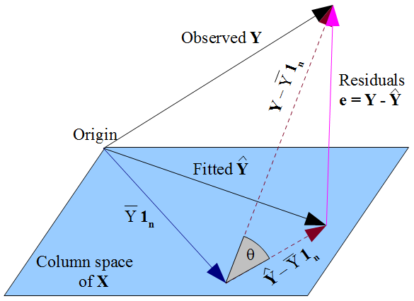
The projection matrix terminology is because \(\mathbf{H}\) represents the orthogonal (i.e., perpendicular) projection of \(\mathbf{Y}\) onto the column space of \(\mathbf{X}\). From our least squares approach, we can think of this as representing the distance that is minimized from our observed to predicted outcome when averaged across all observations. From StackExchange we see an visual representation of this: