This page is part of the University of Colorado-Anschutz Medical Campus’ BIOS 6618 Recitation collection. To view other questions, you can view the BIOS 6618 Recitation collection page or use the search bar to look for keywords.
Polynomial Regression
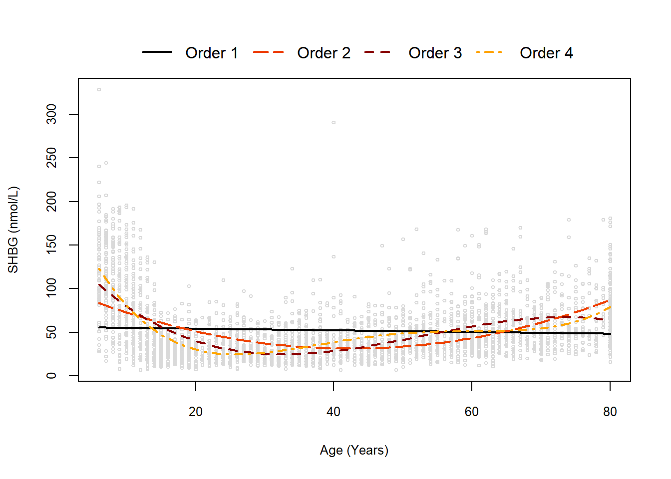
As a motivating example, let’s consider a example from the NHANES 2015-2016 cycle. We are interested in the association between sex hormone binding globulin (SHBG) and age in years for males 6-80 years old from the NHANES 2015-2016 cycle (\(n=3390\) with SHBG). Here we will fit our models using the poly() function with raw=T to mimic a model with higher order terms:
Our simple linear regression model (i.e., a polynomial regression with order 1), is easy to interpret and follows our usual pattern: For a 1 year increase in age, SHBG significantly decreases on average by 0.095 nmol/L (95% CI: 0.042 to 0.148 nmol/L decrease; p<0.001).
However, the interpretations of any models with higher order terms is made far more challenging. Now, the expected change in our outcome will also depend on the value of both \(X\) and \(X^2\) since \(X=20 \implies X^2=400\) which is not an equivalent change to \(X=60 \implies X^2=3600\). In other words, a one-unit increase in age will have different effects depending on the starting point given its non-linear trend over age.
Making it a “brief, but complete” interpretation is a little more challenging since we cannot meaningful interpret the beta coefficients and individual p-values are affected by multicollinearity (in this model with raw, not orthogonal, polynomial terms). However, you consider a variety of approaches:
One of the easiest ways to interpret these models is to plot the trend and describe the trends.
Evaluate the overall contribution of the polynomials (e.g., with a partial \(F\)-test).
Describe the predicted outcome at select predictors (e.g., using GLHT; may be challenging if adjusting for other variables since those would also have an influence).
Calculate the local/global min max, estimate inflection points, or estimate rates of change using calculus.
Calculus in R
Consider our quadratic polynomial. We can estimate the min/max point by taking the first order derivative with respect to \(X\) of our model and setting it equal to 0, then solving for \(X\):
\[\begin{align*}
\hat{Y} = f(X) &= 102.362 + -3.351 X + 0.039 X^2 \\
f'(X) &= -3.351 + 2 \times 0.039 X = -3.351 + 0.078 X \\
0 &= -3.351 + 0.078 X \implies X = \frac{3.351}{0.078} = 42.96
\end{align*}\]
If we plug this back into our regression equation we get the predicted minimum: \(\hat{Y} = 102.362 + -3.351(42.96) + 0.039(42.96)^2 = 30.38\) nmol/L of SHBG.
R also has the ability to do this calculus for us:
Code
# first write our expressionf <-expression( 102.362+-3.351*x +0.039* x^2 )# then use the D() function and specify the variable to derive with respect toD(f, 'x')
0.039 * (2 * x) - 3.351
Code
# uniroot() function calculates where it equals 0 given a range of X valuesfind_root <-function(x) eval( D(f,'x') )uniroot(find_root, c(6,80))
More generally, we can use mosaicCalc::Zeros() to find all candidate points:
Code
library(mosaicCalc)# first write our expressions for the first order derivatives, then findZerosf2 <-D( 102.362+-3.351*x +0.039* x^2~ x )findZeros(f2(x) ~ x, xlim =range(6, 80))
# notice that none were found for f4 due to rounding, we can instead use paste0() and pull the coefficients directly:f4_eq <-paste0(coef(mod_poly4)[1], '+', coef(mod_poly4)[2], '*x +', coef(mod_poly4)[3], '*x^2 +', coef(mod_poly4)[4], '*x^3 +', coef(mod_poly4)[5], '*x^4 ~ x')f4_eq # print regression equation with more decimals to check
From these models, we could interpret that the minimum SHBG is expected, on average, at 43 (quadratic), 28.7 (cubic), or 25.9 (cuartic) years old. We could also estimate the minimum (and 95% CI) by plugging it into our regression equation.
Polynomial Regression and Parsimony
When we fit a regression, we want to find a model that avoids under- and over-fitting the data. Further, we also want to consider the parsimony of our model (i.e., does it have to be as complex or could it be simpler?).
Parsimony in the context of polynomial regression means considering models with fewer higher order terms both to avoid overfitting and having extra, potentially unnecessary, coefficients in our model.
The evaluation of parsimony is often more subjective, but we can use quantitative approaches to determine how many polynomial terms are statistically justified as a starting place.
Partial F-test on Raw Polynomials
If we fit models on our raw polynomials, we may have concerns about collinearity, which could make it challenging to identify the appropriate number of terms.
Let’s start by fitting a sequence of models and running partial F-tests:
Analysis of Variance Table

Model  1: SHBG ~ RIDAGEYR
Model  2: SHBG ~ poly(RIDAGEYR, 2, raw = T)
Model  3: SHBG ~ poly(RIDAGEYR, 3, raw = T)
Model  4: SHBG ~ poly(RIDAGEYR, 4, raw = T)
Model  5: SHBG ~ poly(RIDAGEYR, 5, raw = T)
Model  6: SHBG ~ poly(RIDAGEYR, 6, raw = T)
Model  7: SHBG ~ poly(RIDAGEYR, 7, raw = T)
Model  8: SHBG ~ poly(RIDAGEYR, 8, raw = T)
Model  9: SHBG ~ poly(RIDAGEYR, 9, raw = T)
Model 10: SHBG ~ poly(RIDAGEYR, 10, raw = T)
Model 11: SHBG ~ poly(RIDAGEYR, 11, raw = T)
   Res.Df     RSS Df Sum of Sq         F    Pr(>F)
1    3388 4286690
2    3387 3276833  1   1009857 1351.0353 < 2.2e-16 ***
3    3386 2873485  1    403348  539.6180 < 2.2e-16 ***
4    3385 2618205  1    255281  341.5269 < 2.2e-16 ***
5    3384 2573535  1     44670   59.7615 1.403e-14 ***
6    3383 2558283  1     15252   20.4048 6.482e-06 ***
7    3382 2550263  1      8020   10.7289  0.001065 **
8    3381 2537447  1     12817   17.1467 3.545e-05 ***
9    3380 2529858  1      7589   10.1524  0.001454 **
10   3379 2525059  1      4799    6.4198  0.011330 *
11   3378 2524950  1       109    0.1465  0.701973
---
Signif. codes:  0 '***' 0.001 '**' 0.01 '*' 0.05 '.' 0.1 ' ' 1
Based on these comparisons, it seems that a model with order 10 is considered the “best”.
Lack-of-Fit F-test
When we have replicate observations at each level, we can also estimate the pure versus model error and use it to identify the number of polynomial terms. In the case of our NHANES data, age is only provided as a whole number and we could assume we have lots of categorical data:
 Order 1  Order 2  Order 3  Order 4  Order 5  Order 6  Order 7  Order 8
  0.0000   0.0000   0.0000   0.0000   0.0001   0.0044   0.0234   0.2086
 Order 9 Order 10 Order 11
  0.4763   0.6655   0.6374
Our results indicate that an octic (order 8) polynomial regression is not significantly better than a septic (order 7) polynomial regression. However, the septic (order 7) is better than the sextic (order 6).
This differs from our approach using just raw polynomials, where we chose a more complex order 10 model as “best”.
Orthogonal Polynomial Contrasts
An approach we alluded to, but didn’t delve into details, is the construction of orthogonal polynomial contrasts which remove the correlation between polynomial terms. While the math behind it is a bit lengthy, it is fairly easy to implement in R by removing our raw=T argument (or setting equal to the default FALSE) from poly():
Call:
lm(formula = SHBG ~ poly(RIDAGEYR, 11, raw = F), data = dat)

Residuals:
    Min      1Q  Median      3Q     Max
-100.74  -15.81   -4.69   10.99  254.05

Coefficients:
                               Estimate Std. Error t value Pr(>|t|)
(Intercept)                     52.2391     0.4696 111.250  < 2e-16 ***
poly(RIDAGEYR, 11, raw = F)1  -125.7103    27.3399  -4.598 4.42e-06 ***
poly(RIDAGEYR, 11, raw = F)2  1004.9164    27.3399  36.756  < 2e-16 ***
poly(RIDAGEYR, 11, raw = F)3  -635.0966    27.3399 -23.230  < 2e-16 ***
poly(RIDAGEYR, 11, raw = F)4   505.2531    27.3399  18.480  < 2e-16 ***
poly(RIDAGEYR, 11, raw = F)5  -211.3525    27.3399  -7.731 1.40e-14 ***
poly(RIDAGEYR, 11, raw = F)6   123.4989    27.3399   4.517 6.48e-06 ***
poly(RIDAGEYR, 11, raw = F)7    89.5518    27.3399   3.276  0.00107 **
poly(RIDAGEYR, 11, raw = F)8  -113.2105    27.3399  -4.141 3.54e-05 ***
poly(RIDAGEYR, 11, raw = F)9    87.1125    27.3399   3.186  0.00145 **
poly(RIDAGEYR, 11, raw = F)10  -69.2721    27.3399  -2.534  0.01133 *
poly(RIDAGEYR, 11, raw = F)11   10.4627    27.3399   0.383  0.70197
---
Signif. codes:  0 '***' 0.001 '**' 0.01 '*' 0.05 '.' 0.1 ' ' 1

Residual standard error: 27.34 on 3378 degrees of freedom
Multiple R-squared:  0.4131,    Adjusted R-squared:  0.4112
F-statistic: 216.2 on 11 and 3378 DF,  p-value: < 2.2e-16
We see that the 11th order polynomial is the first to have a p-value >0.05. This agrees with our raw polynomial calculation that Order 10 would be “best”.
With the correlation removed between our predictors, we can also see that a sequence of F-tests for adding each higher order term results in the same p-values:
Code
# print ANOVA comparisons adding 1 higher orthogonal term, notice p-values match those from the regression coefficient table for mod_orth11anova(mod_orth1,mod_orth2,mod_orth3,mod_orth4,mod_orth5,mod_orth6,mod_orth7,mod_orth8,mod_orth9,mod_orth10,mod_orth11)
Analysis of Variance Table

Model  1: SHBG ~ poly(RIDAGEYR, 1, raw = F)
Model  2: SHBG ~ poly(RIDAGEYR, 2, raw = F)
Model  3: SHBG ~ poly(RIDAGEYR, 3, raw = F)
Model  4: SHBG ~ poly(RIDAGEYR, 4, raw = F)
Model  5: SHBG ~ poly(RIDAGEYR, 5, raw = F)
Model  6: SHBG ~ poly(RIDAGEYR, 6, raw = F)
Model  7: SHBG ~ poly(RIDAGEYR, 7, raw = F)
Model  8: SHBG ~ poly(RIDAGEYR, 8, raw = F)
Model  9: SHBG ~ poly(RIDAGEYR, 9, raw = F)
Model 10: SHBG ~ poly(RIDAGEYR, 10, raw = F)
Model 11: SHBG ~ poly(RIDAGEYR, 11, raw = F)
   Res.Df     RSS Df Sum of Sq         F    Pr(>F)
1    3388 4286690
2    3387 3276833  1   1009857 1351.0353 < 2.2e-16 ***
3    3386 2873485  1    403348  539.6180 < 2.2e-16 ***
4    3385 2618205  1    255281  341.5269 < 2.2e-16 ***
5    3384 2573535  1     44670   59.7615 1.403e-14 ***
6    3383 2558283  1     15252   20.4048 6.482e-06 ***
7    3382 2550263  1      8020   10.7289  0.001065 **
8    3381 2537447  1     12817   17.1467 3.545e-05 ***
9    3380 2529858  1      7589   10.1524  0.001454 **
10   3379 2525059  1      4799    6.4198  0.011330 *
11   3378 2524950  1       109    0.1465  0.701973
---
Signif. codes:  0 '***' 0.001 '**' 0.01 '*' 0.05 '.' 0.1 ' ' 1
However, if we did a series of partial F-tests comparing to our saturated pure fit model (mod_pure), we’d arrive at the same conclusion as the lack-of-fit \(F\)-test that a model with order 7 is “best”:
 Order 1  Order 2  Order 3  Order 4  Order 5  Order 6  Order 7  Order 8
  0.0000   0.0000   0.0000   0.0000   0.0001   0.0044   0.0234   0.2086
 Order 9 Order 10 Order 11
  0.4763   0.6655   0.6374
Here, since we are comparing to the saturated model, we can be fairly confident that order 7 may be best. If we did not have a saturated model (e.g., no replicates), we may have chosen the order 10 as optimal based on the orthogonal polynomials (and potentially decided a lower order based on parsimony).
Which Model to Use?
We saw that the raw polynomial approach suggested a model with Order 10, and that both saturated or orthogonal polynomial approaches identified a model with Order 7. Both of these are quite high orders. We may also wish to evaluate other summaries, like the adjusted \(R^2\) value:
Code
rawr2 <-c('Order 1'=summary(mod_lm)$adj.r.squared, 'Order 2'=summary(mod_poly2)$adj.r.squared, 'Order 3'=summary(mod_poly3)$adj.r.squared, 'Order 4'=summary(mod_poly4)$adj.r.squared, 'Order 5'=summary(mod_poly5)$adj.r.squared, 'Order 6'=summary(mod_poly6)$adj.r.squared, 'Order 7'=summary(mod_poly7)$adj.r.squared, 'Order 8'=summary(mod_poly8)$adj.r.squared, 'Order 9'=summary(mod_poly9)$adj.r.squared, 'Order 10'=summary(mod_poly10)$adj.r.squared, 'Order 11'=summary(mod_poly11)$adj.r.squared)ortr2 <-c('Orth Order 1'=summary(mod_orth1)$adj.r.squared, 'Orth Order 2'=summary(mod_orth2)$adj.r.squared, 'Orth Order 3'=summary(mod_orth3)$adj.r.squared, 'Orth Order 4'=summary(mod_orth4)$adj.r.squared, 'Orth Order 5'=summary(mod_orth5)$adj.r.squared, 'Orth Order 6'=summary(mod_orth6)$adj.r.squared, 'Orth Order 7'=summary(mod_orth7)$adj.r.squared, 'Orth Order 8'=summary(mod_orth8)$adj.r.squared, 'Orth Order 9'=summary(mod_orth9)$adj.r.squared, 'Orth Order 10'=summary(mod_orth10)$adj.r.squared, 'Orth Order 11'=summary(mod_orth11)$adj.r.squared)rbind('Raw'= rawr2, 'Orthogonal'= ortr2)
               Order 1   Order 2   Order 3   Order 4   Order 5   Order 6
Raw        0.003378928 0.2379376 0.3315431 0.3907489 0.4009665 0.4043407
Orthogonal 0.003378928 0.2379376 0.3315431 0.3907489 0.4009665 0.4043407
             Order 7   Order 8   Order 9  Order 10  Order 11
Raw        0.4060323 0.4088426 0.4104361 0.4113803 0.4112316
Orthogonal 0.4060323 0.4088426 0.4104361 0.4113803 0.4112316
We can note 2 things from these \(R^2_{adj}\) results:
The estimated percent of variability explained by each raw and orthogonal polynomial model of the same order are identical! This is because while the orthogonal polynomials transform our predictors to remove collinearity, the same data/information is included in the model.
It appears that after Order 4, the jumps in \(R^2_{adj}\) get smaller and smaller. This may suggest a model with Order 4 may be sufficient.
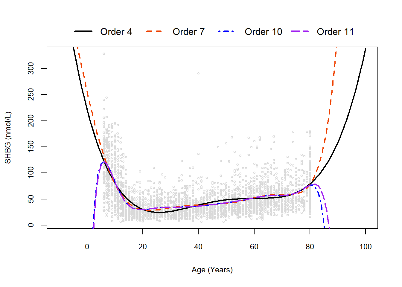
To evaluate, let’s compare the some models while also illustrating the dangers of extrapolation:
First, note extrapolation beyond our observed data quickly gets crazy and shouldn’t be done for our polynomial models.
Second, I think the choice of “best” Order 4 or Order 7 depends on our own belief of how well it fits the data without being potentially overfit. Further, Orders 10 and 11 are quite similar to Order 7, so even if we had used a method and chosen Order 10, it wouldn’t be wrong (just overly complex).
Other Modeling Approaches
There are also other modeling strategies that may be helpful beyond polynomial regression and are covered in some other lectures:
Spline modeling provides more flexibility for the trends (but is still hard to interpret)
Piecewise regression models are more interpretable and identify break/changepoints where the trend changes/shifts
Source Code
---title: "Interpreting Polynomial Regression Models, Selecting Your Highest Order Polynomial Term, and Calculus in R"author: name: Alex Kaizer roles: "Instructor" affiliation: University of Colorado-Anschutz Medical Campustoc: truetoc_float: truetoc-location: leftformat: html: code-fold: show code-overflow: wrap code-tools: true---```{r, echo=F, message=F, warning=F}library(kableExtra)library(dplyr)```This page is part of the University of Colorado-Anschutz Medical Campus' [BIOS 6618 Recitation](/recitation/index.qmd) collection. To view other questions, you can view the [BIOS 6618 Recitation](/recitation/index.qmd) collection page or use the search bar to look for keywords.# Polynomial RegressionAs a motivating example, let's consider a example from the NHANES 2015-2016 cycle. We are interested in the association between sex hormone binding globulin (SHBG) and age in years for males 6-80 years old from the NHANES 2015-2016 cycle ($n=3390$ with SHBG). Here we will fit our models using the `poly()` function with `raw=T` to mimic a model with higher order terms:```{r, class.source = 'fold-hide'}#| code-fold: truedat <-read.csv('../../.data/nhanes1516_sexhormone.csv')dat <- dat[which(dat$MALE==T),]dat <- dat[!is.na(dat$SHBG),]plot(x=dat$RIDAGEYR, y=dat$SHBG, xlab='Age (Years)', ylab='SHBG (nmol/L)', col='gray85', cex.lab=0.8, cex.axis=0.8, cex=0.5)mod_lm <-lm(SHBG~RIDAGEYR, data=dat)mod_poly2 <-lm(SHBG~poly(RIDAGEYR,2, raw=T), data=dat)mod_poly3 <-lm(SHBG~poly(RIDAGEYR,3, raw=T), data=dat)mod_poly4 <-lm(SHBG~poly(RIDAGEYR,4, raw=T), data=dat)age <-6:80lines(x=age, y=predict(mod_lm, newdata=data.frame(RIDAGEYR=age)), lwd=2, col='black')lines(x=age, y=predict(mod_poly2, newdata=data.frame(RIDAGEYR=age)), lwd=2, col='orangered2', lty=5)lines(x=age, y=predict(mod_poly3, newdata=data.frame(RIDAGEYR=age)), lwd=2, col='red4', lty=2)lines(x=age, y=predict(mod_poly4, newdata=data.frame(RIDAGEYR=age)), lwd=2, col='orange', lty=4)legend('top', horiz=T, bty='n', xpd=T, inset=-0.15, lty=c(1,5,2,4), lwd=c(2,2,2,2), legend=c('Order 1','Order 2','Order 3','Order 4'), col=c('black','orangered2','red4','orange'))```## Interpretation of TrendsLet's examine the model fit for each of the models:1. $\hat{Y} = 55.903 + -0.095 X$2. $\hat{Y} = 102.362 + -3.351 X + 0.039 X^2$3. $\hat{Y} = 152.581 + -9.177 X + 0.203 X^2 + -0.001 X^3$4. $\hat{Y} = 221.308 + -20.371 X + 0.730 X^2 + -0.011 X^3 + 0.00005 X^4$Our simple linear regression model (i.e., a polynomial regression with order 1), is easy to interpret and follows our usual pattern: *For a 1 year increase in age, SHBG significantly decreases on average by 0.095 nmol/L (95% CI: 0.042 to 0.148 nmol/L decrease; p<0.001).*However, the interpretations of any models with higher order terms is made far more challenging. Now, the expected change in our outcome will also depend on the value of both $X$ and $X^2$ since $X=20 \implies X^2=400$ which is not an equivalent change to $X=60 \implies X^2=3600$. In other words, a one-unit increase in age will have different effects depending on the starting point given its *non-linear* trend over age.Making it a "brief, but complete" interpretation is a little more challenging since we cannot meaningful interpret the beta coefficients and individual p-values are affected by multicollinearity (in this model with raw, not orthogonal, polynomial terms). However, you consider a variety of approaches:- One of the easiest ways to interpret these models is to plot the trend and describe the trends.- Evaluate the overall contribution of the polynomials (e.g., with a partial $F$-test).- Describe the predicted outcome at select predictors (e.g., using GLHT; may be challenging if adjusting for other variables since those would also have an influence).- Calculate the local/global min max, estimate inflection points, or estimate rates of change using calculus.### Calculus in RConsider our quadratic polynomial. We can estimate the min/max point by taking the first order derivative with respect to $X$ of our model and setting it equal to 0, then solving for $X$:$$\begin{align*} \hat{Y} = f(X) &= 102.362 + -3.351 X + 0.039 X^2 \\f'(X) &= -3.351 + 2 \times 0.039 X = -3.351 + 0.078 X \\0 &= -3.351 + 0.078 X \implies X = \frac{3.351}{0.078} = 42.96\end{align*}$$If we plug this back into our regression equation we get the predicted minimum: $\hat{Y} = 102.362 + -3.351(42.96) + 0.039(42.96)^2 = 30.38$ nmol/L of SHBG.R also has the ability to do this calculus for us:```{r}# first write our expressionf <-expression( 102.362+-3.351*x +0.039* x^2 )# then use the D() function and specify the variable to derive with respect toD(f, 'x')# uniroot() function calculates where it equals 0 given a range of X valuesfind_root <-function(x) eval( D(f,'x') )uniroot(find_root, c(6,80))```More generally, we can use `mosaicCalc::Zeros()` to find all candidate points:```{r, warning=F, message=F}library(mosaicCalc)# first write our expressions for the first order derivatives, then findZerosf2 <-D( 102.362+-3.351*x +0.039* x^2~ x )findZeros(f2(x) ~ x, xlim =range(6, 80))f3 <-D( 152.581+-9.177*x +0.203*x^2+-0.001*x^3~ x )findZeros(f3(x) ~ x, xlim =range(6, 80))f4 <-D( 221.308+-20.371*x +0.730*x^2+-0.011*x^3+0.00005*x^4~ x )findZeros(f4(x) ~ x, xlim =range(6, 80))# notice that none were found for f4 due to rounding, we can instead use paste0() and pull the coefficients directly:f4_eq <-paste0(coef(mod_poly4)[1], '+', coef(mod_poly4)[2], '*x +', coef(mod_poly4)[3], '*x^2 +', coef(mod_poly4)[4], '*x^3 +', coef(mod_poly4)[5], '*x^4 ~ x')f4_eq # print regression equation with more decimals to checkf4_coef <-D( as.formula(f4_eq) )findZeros(f4_coef(x) ~ x, xlim =range(6, 80))```From these models, we could interpret that the minimum SHBG is expected, on average, at 43 (quadratic), 28.7 (cubic), or 25.9 (cuartic) years old. We could also estimate the minimum (and 95% CI) by plugging it into our regression equation.## Polynomial Regression and ParsimonyWhen we fit a regression, we want to find a model that avoids under- and over-fitting the data. Further, we also want to consider the parsimony of our model (i.e., does it have to be as complex or could it be simpler?).Parsimony in the context of polynomial regression means considering models with fewer higher order terms both to avoid overfitting and having extra, potentially unnecessary, coefficients in our model.The evaluation of parsimony is often more subjective, but we can use quantitative approaches to determine how many polynomial terms are statistically justified as a starting place.### Partial F-test on Raw PolynomialsIf we fit models on our raw polynomials, we may have concerns about collinearity, which could make it challenging to identify the appropriate number of terms.Let's start by fitting a sequence of models and running partial F-tests:```{r}mod_lm <-lm(SHBG~RIDAGEYR, data=dat)mod_poly2 <-lm(SHBG~poly(RIDAGEYR,2, raw=T), data=dat)mod_poly3 <-lm(SHBG~poly(RIDAGEYR,3, raw=T), data=dat)mod_poly4 <-lm(SHBG~poly(RIDAGEYR,4, raw=T), data=dat)mod_poly5 <-lm(SHBG~poly(RIDAGEYR,5, raw=T), data=dat)mod_poly6 <-lm(SHBG~poly(RIDAGEYR,6, raw=T), data=dat)mod_poly7 <-lm(SHBG~poly(RIDAGEYR,7, raw=T), data=dat)mod_poly8 <-lm(SHBG~poly(RIDAGEYR,8, raw=T), data=dat)mod_poly9 <-lm(SHBG~poly(RIDAGEYR,9, raw=T), data=dat)mod_poly10 <-lm(SHBG~poly(RIDAGEYR,10, raw=T), data=dat)mod_poly11 <-lm(SHBG~poly(RIDAGEYR,11, raw=T), data=dat)# partial F-tests (i.e., equivalent to observing coefficients and analyzing highest order t-statistic and p-value)anova(mod_lm,mod_poly2,mod_poly3,mod_poly4,mod_poly5,mod_poly6,mod_poly7,mod_poly8,mod_poly9,mod_poly10,mod_poly11)```Based on these comparisons, it seems that a model with order 10 is considered the "best".### Lack-of-Fit F-testWhen we have replicate observations at each level, we can also estimate the pure versus model error and use it to identify the number of polynomial terms. In the case of our NHANES data, age is only provided as a whole number and we could assume we have lots of categorical data:```{r}# fit saturated modelmod_pure <-lm(SHBG ~as.factor(RIDAGEYR), data=dat)# save p-values from partial F-testsp1 <-anova(mod_pure, mod_lm)["Pr(>F)"][2,1]p2 <-anova(mod_pure, mod_poly2)["Pr(>F)"][2,1]p3 <-anova(mod_pure, mod_poly3)["Pr(>F)"][2,1]p4 <-anova(mod_pure, mod_poly4)["Pr(>F)"][2,1]p5 <-anova(mod_pure, mod_poly5)["Pr(>F)"][2,1]p6 <-anova(mod_pure, mod_poly6)["Pr(>F)"][2,1]p7 <-anova(mod_pure, mod_poly7)["Pr(>F)"][2,1]p8 <-anova(mod_pure, mod_poly8)["Pr(>F)"][2,1]p9 <-anova(mod_pure, mod_poly9)["Pr(>F)"][2,1]p10 <-anova(mod_pure, mod_poly10)["Pr(>F)"][2,1]p11 <-anova(mod_pure, mod_poly11)["Pr(>F)"][2,1]# print p-valuesround(c('Order 1'=p1, 'Order 2'=p2, 'Order 3'=p3, 'Order 4'=p4, 'Order 5'=p5, 'Order 6'=p6, 'Order 7'=p7, 'Order 8'=p8, 'Order 9'=p9, 'Order 10'=p10, 'Order 11'=p11),4)```Our results indicate that an octic (order 8) polynomial regression is not significantly better than a septic (order 7) polynomial regression. However, the septic (order 7) is better than the sextic (order 6). This differs from our approach using just raw polynomials, where we chose a more complex order 10 model as "best".### Orthogonal Polynomial ContrastsAn approach we alluded to, but didn't delve into details, is the construction of orthogonal polynomial contrasts which remove the correlation between polynomial terms. While the math behind it is a bit lengthy, it is fairly easy to implement in `R` by removing our `raw=T` argument (or setting equal to the default `FALSE`) from `poly()`:```{r}mod_orth1 <-lm( SHBG~poly(RIDAGEYR,1, raw=F), data=dat)mod_orth2 <-lm( SHBG~poly(RIDAGEYR,2, raw=F), data=dat)mod_orth3 <-lm( SHBG~poly(RIDAGEYR,3, raw=F), data=dat)mod_orth4 <-lm( SHBG~poly(RIDAGEYR,4, raw=F), data=dat)mod_orth5 <-lm( SHBG~poly(RIDAGEYR,5, raw=F), data=dat)mod_orth6 <-lm( SHBG~poly(RIDAGEYR,6, raw=F), data=dat)mod_orth7 <-lm( SHBG~poly(RIDAGEYR,7, raw=F), data=dat)mod_orth8 <-lm( SHBG~poly(RIDAGEYR,8, raw=F), data=dat)mod_orth9 <-lm( SHBG~poly(RIDAGEYR,9, raw=F), data=dat)mod_orth10 <-lm( SHBG~poly(RIDAGEYR,10, raw=F), data=dat)mod_orth11 <-lm( SHBG~poly(RIDAGEYR,11, raw=F), data=dat)# print summary of Order 11 polynomial regressionsummary(mod_orth11)```We see that the 11th order polynomial is the first to have a p-value >0.05. This agrees with our raw polynomial calculation that Order 10 would be "best". With the correlation removed between our predictors, we can also see that a sequence of F-tests for adding each higher order term results in the same p-values:```{r}# print ANOVA comparisons adding 1 higher orthogonal term, notice p-values match those from the regression coefficient table for mod_orth11anova(mod_orth1,mod_orth2,mod_orth3,mod_orth4,mod_orth5,mod_orth6,mod_orth7,mod_orth8,mod_orth9,mod_orth10,mod_orth11)```However, if we did a series of partial F-tests comparing to our saturated pure fit model (`mod_pure`), we'd arrive at the same conclusion as the lack-of-fit $F$-test that a model with order 7 is "best":```{r}o1 <-anova(mod_pure, mod_orth1)["Pr(>F)"][2,1]o2 <-anova(mod_pure, mod_orth2)["Pr(>F)"][2,1]o3 <-anova(mod_pure, mod_orth3)["Pr(>F)"][2,1]o4 <-anova(mod_pure, mod_orth4)["Pr(>F)"][2,1]o5 <-anova(mod_pure, mod_orth5)["Pr(>F)"][2,1]o6 <-anova(mod_pure, mod_orth6)["Pr(>F)"][2,1]o7 <-anova(mod_pure, mod_orth7)["Pr(>F)"][2,1]o8 <-anova(mod_pure, mod_orth8)["Pr(>F)"][2,1]o9 <-anova(mod_pure, mod_orth9)["Pr(>F)"][2,1]o10 <-anova(mod_pure, mod_orth10)["Pr(>F)"][2,1]o11 <-anova(mod_pure, mod_orth11)["Pr(>F)"][2,1]round(c('Order 1'=o1, 'Order 2'=o2, 'Order 3'=o3, 'Order 4'=o4, 'Order 5'=o5, 'Order 6'=o6, 'Order 7'=o7, 'Order 8'=o8, 'Order 9'=o9, 'Order 10'=o10, 'Order 11'=o11),4)```Here, since we are comparing to the saturated model, we can be fairly confident that order 7 may be best. If we did not have a saturated model (e.g., no replicates), we may have chosen the order 10 as optimal based on the orthogonal polynomials (and potentially decided a lower order based on parsimony).### Which Model to Use?We saw that the raw polynomial approach suggested a model with Order 10, and that both saturated or orthogonal polynomial approaches identified a model with Order 7. Both of these are quite high orders. We may also wish to evaluate other summaries, like the adjusted $R^2$ value:```{r, class.source = 'fold-hide'}#| code-fold: truerawr2 <-c('Order 1'=summary(mod_lm)$adj.r.squared, 'Order 2'=summary(mod_poly2)$adj.r.squared, 'Order 3'=summary(mod_poly3)$adj.r.squared, 'Order 4'=summary(mod_poly4)$adj.r.squared, 'Order 5'=summary(mod_poly5)$adj.r.squared, 'Order 6'=summary(mod_poly6)$adj.r.squared, 'Order 7'=summary(mod_poly7)$adj.r.squared, 'Order 8'=summary(mod_poly8)$adj.r.squared, 'Order 9'=summary(mod_poly9)$adj.r.squared, 'Order 10'=summary(mod_poly10)$adj.r.squared, 'Order 11'=summary(mod_poly11)$adj.r.squared)ortr2 <-c('Orth Order 1'=summary(mod_orth1)$adj.r.squared, 'Orth Order 2'=summary(mod_orth2)$adj.r.squared, 'Orth Order 3'=summary(mod_orth3)$adj.r.squared, 'Orth Order 4'=summary(mod_orth4)$adj.r.squared, 'Orth Order 5'=summary(mod_orth5)$adj.r.squared, 'Orth Order 6'=summary(mod_orth6)$adj.r.squared, 'Orth Order 7'=summary(mod_orth7)$adj.r.squared, 'Orth Order 8'=summary(mod_orth8)$adj.r.squared, 'Orth Order 9'=summary(mod_orth9)$adj.r.squared, 'Orth Order 10'=summary(mod_orth10)$adj.r.squared, 'Orth Order 11'=summary(mod_orth11)$adj.r.squared)rbind('Raw'= rawr2, 'Orthogonal'= ortr2)```We can note 2 things from these $R^2_{adj}$ results:1. The estimated percent of variability explained by each raw and orthogonal polynomial model of the same order *are identical*! This is because while the orthogonal polynomials transform our predictors to remove collinearity, the same data/information is included in the model.2. It appears that after Order 4, the jumps in $R^2_{adj}$ get smaller and smaller. This may suggest a model with Order 4 may be sufficient.To evaluate, let's compare the some models while also illustrating the dangers of extrapolation:```{r, class.source = 'fold-hide'}#| code-fold: trueplot(x=dat$RIDAGEYR, y=dat$SHBG, xlab='Age (Years)', ylab='SHBG (nmol/L)', col='gray85', cex.lab=0.8, cex.axis=0.8, cex=0.5, xlim=c(-10,100))age <--10:100lines(x=age, y=predict(mod_poly4, newdata=data.frame(RIDAGEYR=age)), lwd=2, col='black', lty=1)lines(x=age, y=predict(mod_poly7, newdata=data.frame(RIDAGEYR=age)), lwd=2, col='orangered2', lty=2)lines(x=age, y=predict(mod_poly10, newdata=data.frame(RIDAGEYR=age)), lwd=2, col='blue', lty=4)lines(x=age, y=predict(mod_poly11, newdata=data.frame(RIDAGEYR=age)), lwd=2, col='purple', lty=5)legend('top', horiz=T, bty='n', xpd=T, inset=-0.15, lty=c(1,2,4,5), lwd=c(2,2,2,2), legend=c('Order 4','Order 7','Order 10','Order 11'), col=c('black','orangered2','blue','purple'))```First, note extrapolation beyond our observed data quickly gets crazy and shouldn't be done for our polynomial models.Second, I think the choice of "best" Order 4 or Order 7 depends on our own belief of how well it fits the data without being potentially overfit. Further, Orders 10 and 11 are quite similar to Order 7, so even if we had used a method and chosen Order 10, it wouldn't be wrong (just overly complex).## Other Modeling ApproachesThere are also other modeling strategies that may be helpful beyond polynomial regression and are covered in some other lectures:- Spline modeling provides more flexibility for the trends (but is still hard to interpret)- Piecewise regression models are more interpretable and identify break/changepoints where the trend changes/shifts