What Are Some R Packages for Diagnostic Testing Calculations?

Author

Affiliation

Alex Kaizer

University of Colorado-Anschutz Medical Campus

This page is part of the University of Colorado-Anschutz Medical Campus’ BIOS 6618 Recitation collection. To view other questions, you can view the BIOS 6618 Recitation collection page or use the search bar to look for keywords.

Note, this recitation was written in 2022 and packages may have changed.

R Packages for Diagnostic Testing Calculations

There are lots of packages out there that can calculate the diagnostic test summaries. Below I provide a few I use with comments about certain properties.

For illustration purposes, let’s also simulate some data for a prospective cohort study with:

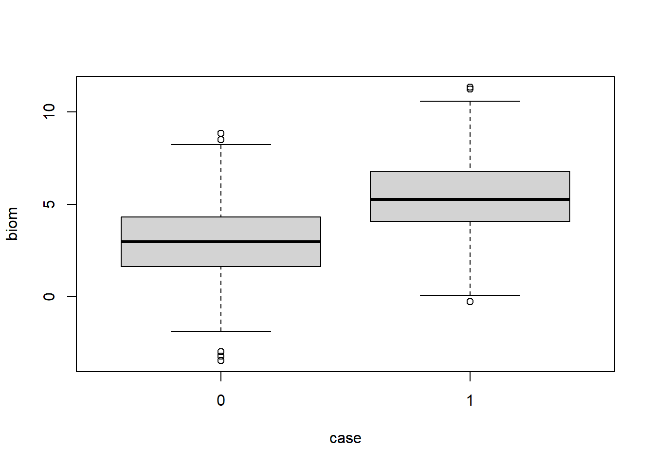
200 participants who develop the condition of interest and have a baseline biomarker measure distributed $N(\mu=5,\sigma=2)$
800 participants who do not develop the condition of interest and have a baseline biomarker measure distributed $N(\mu=3,\sigma=2)$

Code

set.seed(515)

# Make data set to illustrate functions below
diag_dat <- data.frame(
  case = c(rep(1,200), rep(0,800)), # create variable to indicate outcome status
  biom = c(rnorm(200,5,2), rnorm(800,3,2)) # create variable for baseline biomarker measurement
)

Visualizing the data, we see there is overlap in the biomarkers between groups:

Code

boxplot(biom ~ case, data=diag_dat)

We will examine the properties if we use a threshold of >4 to indicate a predicted case versus a control:

Code

# The tricky thing, as we will see below, is we want our table to be ordered similar to our notes so we need to tell R the order so it doesn't use the alpha-numeric default
tab4 <- table(biom_gt4 = factor(diag_dat$biom>4, levels=c(T,F), labels=c(T,F)), truth = factor(diag_dat$case, levels=c(1,0), labels=c(1,0)) )

tab4

        truth
biom_gt4   1   0
   TRUE  152 241
   FALSE  48 559

In the code above we used factor to tell R the order we wanted the table’s results, so it can reflect the structure of the 2x2 table in our notes:

	Case	Control
Test +	a	b
Test -	c	d

If we did not define it, we will end up with the alpha-numeric default ordering that will lead to incorrect interpretations of our summaries:

Code

# Note that if we didn't use something like factor to set the order we end up with:
table(biom_gt4 = diag_dat$biom>4, case = diag_dat$case )

        case
biom_gt4   0   1
   FALSE 559  48
   TRUE  241 152

`epiR` Package

I like the epiR package since it can quickly return summaries based on the provided 2x2 table with confidence intervals (epi.tests gives the diagnostic testing summaries, epi.2x2 provides the OR, RR, etc.):

Code

epiR::epi.tests(tab4)

          Outcome +    Outcome -      Total
Test +          152          241        393
Test -           48          559        607
Total           200          800       1000

Point estimates and 95% CIs:
--------------------------------------------------------------
Apparent prevalence *                  0.39 (0.36, 0.42)
True prevalence *                      0.20 (0.18, 0.23)
Sensitivity *                          0.76 (0.69, 0.82)
Specificity *                          0.70 (0.67, 0.73)
Positive predictive value *            0.39 (0.34, 0.44)
Negative predictive value *            0.92 (0.90, 0.94)
Positive likelihood ratio              2.52 (2.21, 2.88)
Negative likelihood ratio              0.34 (0.27, 0.44)
False T+ proportion for true D- *      0.30 (0.27, 0.33)
False T- proportion for true D+ *      0.24 (0.18, 0.31)
False T+ proportion for T+ *           0.61 (0.56, 0.66)
False T- proportion for T- *           0.08 (0.06, 0.10)
Correctly classified proportion *      0.71 (0.68, 0.74)
--------------------------------------------------------------
* Exact CIs

If we investigate the names, we can also extract the specific estimates and confidence intervals of interest:

Code

# save epiR::epi.tests(tab4) as object
resR <- epiR::epi.tests(tab4)

# check names for returned output
names(resR)

[1] "detail"     "tab"        "method"     "digits"     "conf.level"

Code

# see output for detail
resR$detail

   statistic        est      lower      upper
1         ap 0.39300000 0.36258124  0.4240507
2         tp 0.20000000 0.17562057  0.2261594
3         se 0.76000000 0.69469371  0.8174281
4         sp 0.69875000 0.66564151  0.7303860
5    diag.ac 0.71100000 0.68181223  0.7389396
6    diag.or 7.34508990 5.13510725 10.5061770
7       nndx 2.17983651 1.82543694  2.7751936
8     youden 0.45875000 0.36033522  0.5478140
9     pv.pos 0.38676845 0.33835951  0.4368964
10    pv.neg 0.92092257 0.89652027  0.9411214
11    lr.pos 2.52282158 2.21270687  2.8763994
12    lr.neg 0.34347048 0.26728509  0.4413713
13    p.rout 0.60700000 0.57594932  0.6374188
14     p.rin 0.39300000 0.36258124  0.4240507
15    p.tpdn 0.30125000 0.26961405  0.3343585
16    p.tndp 0.24000000 0.18257190  0.3053063
17    p.dntp 0.61323155 0.56310356  0.6616405
18    p.dptn 0.07907743 0.05887859  0.1034797

Code

# check object type for detail
class( resR$detail )

[1] "data.frame"

Code

# extract sensitivity
resR$detail[ which(resR$detail$statistic == 'se'), ]

  statistic  est     lower     upper
3        se 0.76 0.6946937 0.8174281

Code

# Alternative ways we could extract sensitivity
## Save resR$detail as its own object to avoid lots of $'s
resR_detail <- resR$detail
resR_detail[ which(resR_detail$statistic == 'se'), ]

  statistic  est     lower     upper
3        se 0.76 0.6946937 0.8174281

Code

## Use square brackets to pull statistic from resR$detail
resR$detail[ which(resR$detail[,'statistic'] == 'se'), ]

  statistic  est     lower     upper
3        se 0.76 0.6946937 0.8174281

The limitation of epi.tests is that the negative and positive predictive value summaries are based on the sample prevalence (the function output calls it the “true” prevalence: tprev). If we have a different population prevalence to use, we either have to manually extract the estimates for sensitivity and specificity to use in our formulas, or explore other functions.

NOTE: epiR updated their package so that epi.tests() uses the above approach to extract our statistic(s) of interest. In older versions, you could use something along the lines of resR$rval to produce something like resR$detail. To update to the latest version of the package, you can use install.packages('epiR') or click through options in RStudio.

`caret` Package

The caret package includes functions that can calculate our diagnostic summaries, while also including the population prevalence. There are also multiple ways to provide the data for the functions.

For example, to calculate our sensitivity we can either provide our 2x2 table or the vectors of our results. For the 2x2 table the rows and columns must have the same names, and for the vectors we still need to provide factors:

Code

# make table with same names for row and column
tab4c <- table(biom_gt4 = factor(diag_dat$biom>4, levels=c(T,F), labels=c(1,0)), truth = factor(diag_dat$case, levels=c(1,0), labels=c(1,0)) )

caret::sensitivity(tab4c)

[1] 0.76

Code

# feed in vectors of factor variables instead
caret::sensitivity(factor(diag_dat$biom>4, levels=c(T,F), labels=c(1,0)), factor(diag_dat$case, levels=c(1,0), labels=c(1,0)))

[1] 0.76

For NPV and PPV, we can specify the prevalence (or if we leave it blank it uses the sample estimate):

Code

# Use sample prevalence to compare to epiR output above
caret::posPredValue(tab4c, prevalence=NULL)

[1] 0.3867684

Code

# Specify population prevalence of 10%
caret::posPredValue(tab4c, prevalence=0.1)

[1] 0.2189413

A downside to this approach, however, is there is no automatically provided confidence intervals. We either have to find a formula to use or implement a bootstrap resampling strategy to estimate a confidence interval.

R Packages for Diagnostic Testing Calculations

epiR Package

caret Package

`epiR` Package

`caret` Package