Code
set.seed(1008)
dat1 <- rnorm(n=10, mean=10, sd=3)
hist(dat1, main='Histogram of n=10 from N(10,9)')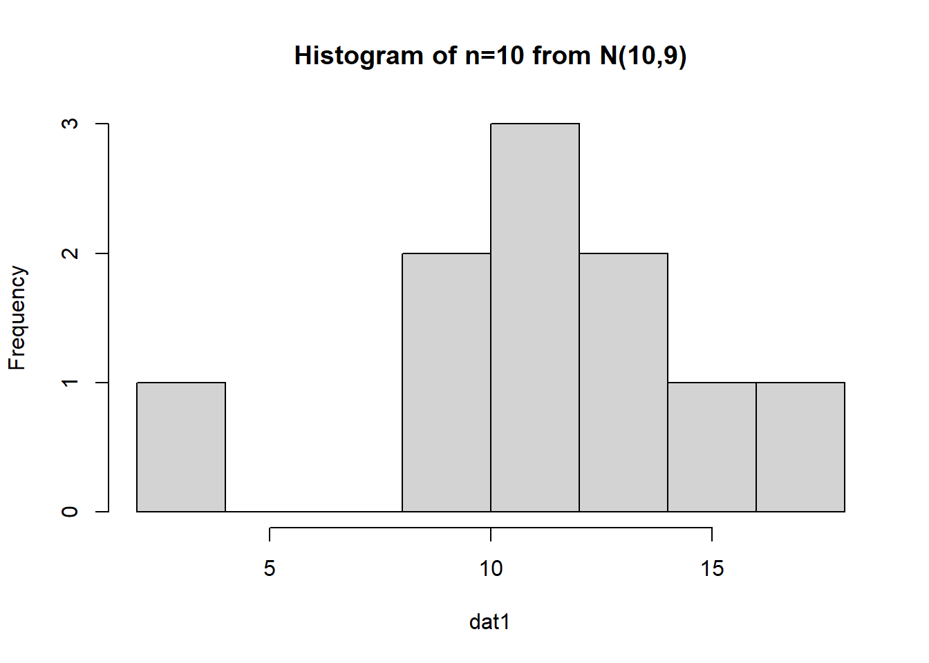
This page is part of the University of Colorado-Anschutz Medical Campus’ BIOS 6618 Recitation collection. To view other questions, you can view the BIOS 6618 Recitation collection page or use the search bar to look for keywords.
What target coverage in our upper and lower tails of our 95% confidence interval would be considered “good”? For example, if we are calculating a 95% confidence interval, based on the normal distribution being symmetric around the mean, we would expect exactly 2.5% coverage in both tails. As a distribution departs from normality, we will start to see coverage that does not nicely meet our expected coverage.
So how bad is too bad? Strictly speaking, if we do not achieve the target coverage the normal percentile method may not be appropriate, and perhaps other methods (e.g., the bootstrap percentile CI) would be more appropriate. But we usually are willing to accept some level of variability (i.e., we introduce some subjectivity). Perhaps being only 0.1% off the coverage is acceptable, or maybe even more.
To illustrate this trade-off, let’s examine bootstraps for the simpler case of estimating the sample mean.
First, let’s examine if we simulate a normal data set with a smaller sample size (\(n=10\)):
set.seed(1008)
dat1 <- rnorm(n=10, mean=10, sd=3)
hist(dat1, main='Histogram of n=10 from N(10,9)')
The data appears to be approximately normal (although with \(n=10\) we may need to use our imagination a bit). Let’s conduct a bootstrap sample with 10,000 bootstrap samples to estimate our 95% CI:
# note, we set our seed above
n <- length(dat1)
B <- 10000
boot_vec <- as.numeric(B)

for(i in 1:B){
  boot_vec[i] <- mean(sample(dat1, n, replace = TRUE) )
}

hist(boot_vec, main='Bootstrap Distribution of Sample Mean, n=10 Normal')
qqnorm(boot_vec); qqline(boot_vec)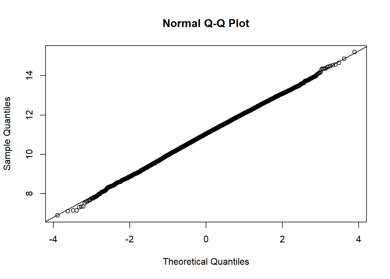
Based on the histogram and QQ plot, the distribution appears mostly normal (as we would expect when we simulate data from a normal distribution and calculate the mean, which we know is exactly distributed normally). The 95% normal percentile interval is
#Lower limit of 95% Normal CI
LL <- mean(boot_vec)-1.96*sd(boot_vec)
LL
[1] 8.940995#Upper limit of 95% Normal CI
UL <- mean(boot_vec)+1.96*sd(boot_vec)
UL[1] 13.10318sum(boot_vec < LL)/B # Coverage of CI at lower end[1] 0.0271sum(boot_vec > UL)/B # Coverage of CI at upper end [1] 0.0221We see here the results are pretty close for coverage! We can also compare to the bootstrap percentile interval:
quantile(boot_vec, c(0.025,0.975)) 2.5% 97.5%
8.904613 13.054325 Here the two intervals are extremely similar, because the coverage is pretty close to our target of 2.5%.
For completeness, we can also calculate the ratio of the bias to the standard error to see if it exceeds ±0.10:
# estimate of accuracy for our bootstrap percentile interval
(mean(boot_vec)-mean(dat1)) / sd(boot_vec)
[1] 0.001938323What if we have a much larger sample that comes from a normal distribution?
set.seed(1021)
dat2 <- rnorm(n=200, mean=10, sd=3)
hist(dat2, main='Histogram of n=200 from N(10,9)')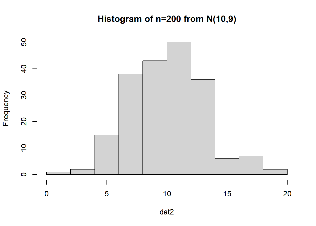
The data appears to be pretty darned normal, but let’s conduct a bootstrap sample with 10,000 bootstrap samples:
# note, we set our seed above
n <- length(dat2)
B <- 10000
boot_vec2 <- as.numeric(B)

for(i in 1:B){
  boot_vec2[i] <- mean(sample(dat2, n, replace = TRUE) )
}

hist(boot_vec2, main='Bootstrap Distribution of Sample Mean, n=200 Normal')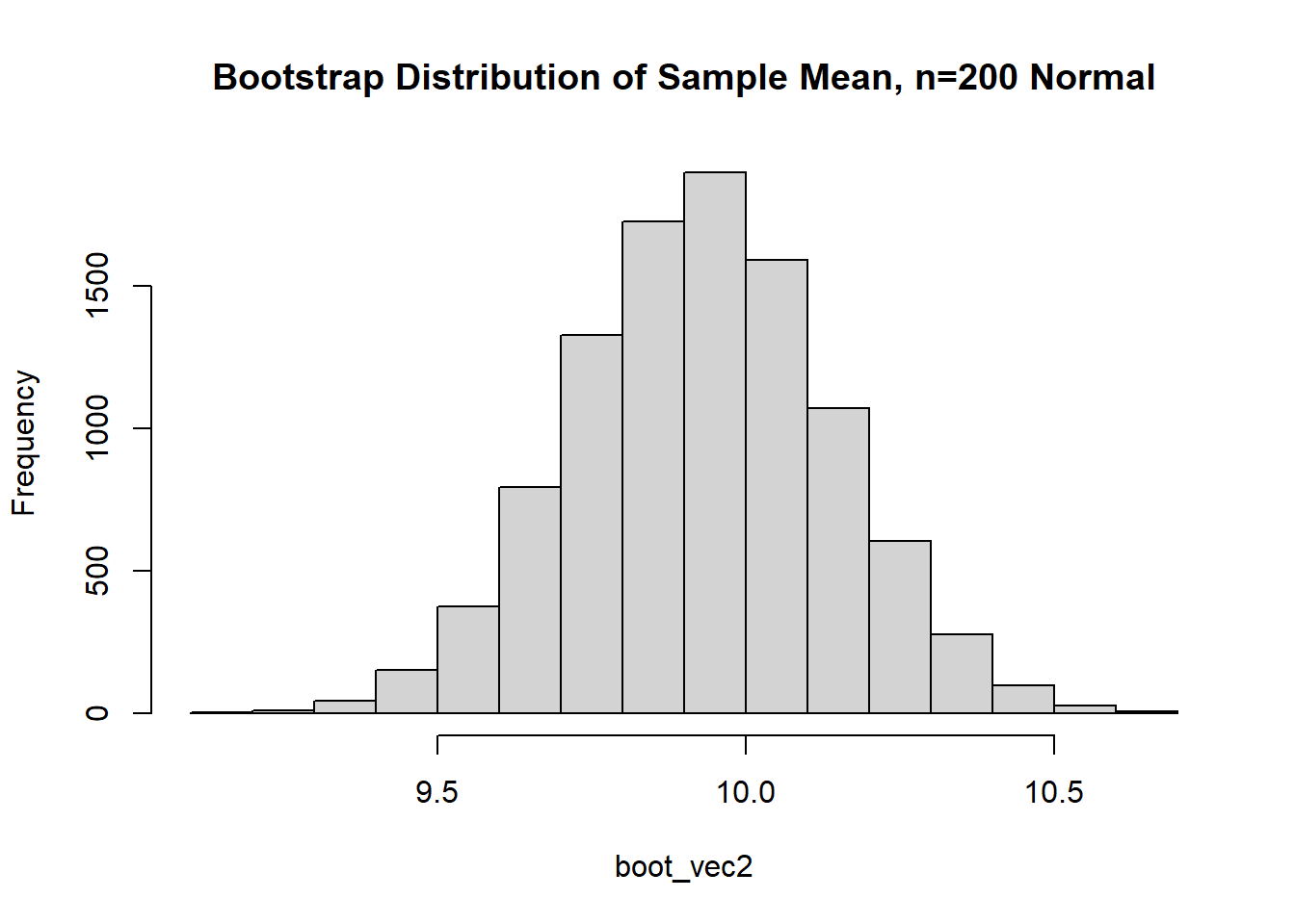
qqnorm(boot_vec2); qqline(boot_vec2)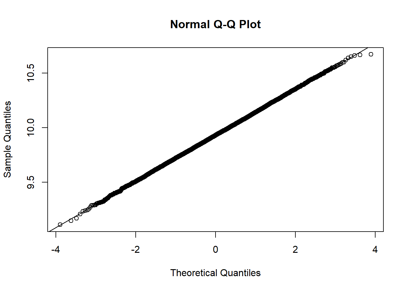
Based on the histogram and QQ plot, the distribution appears extremely normal (as we would expect when we simulate data from a normal distribution and calculate the mean, which we know is exactly distributed normally). The 95% normal percentile interval is
#Lower limit of 95% Normal CI
LL <- mean(boot_vec2)-1.96*sd(boot_vec2)
LL
[1] 9.515987#Upper limit of 95% Normal CI
UL <- mean(boot_vec2)+1.96*sd(boot_vec2)
UL[1] 10.34445sum(boot_vec2 < LL)/B # Coverage of CI at lower end[1] 0.025sum(boot_vec2 > UL)/B # Coverage of CI at upper end [1] 0.0258We see here the results are spot on for the lower limit (LL) and close for the upper limit (UL) coverage! We can also compare to the bootstrap percentile interval:
quantile(boot_vec2, c(0.025,0.975)) 2.5% 97.5%
9.516301 10.346530 Again, the two confidence intervals match pretty closely.
For completeness, we can also calculate the ratio of the bias to the standard error to see if it exceeds ±0.10:
# estimate of accuracy for our bootstrap percentile interval
(mean(boot_vec2)-mean(dat2)) / sd(boot_vec2)
[1] 0.001533928First, let’s examine if we simulate an exponential data set with a smaller sample size (\(n=10\)):
set.seed(1008)
dat3 <- rexp(n=10, rate=1/3)
hist(dat3, main='Histogram of n=10 from Exp(rate=1/3)')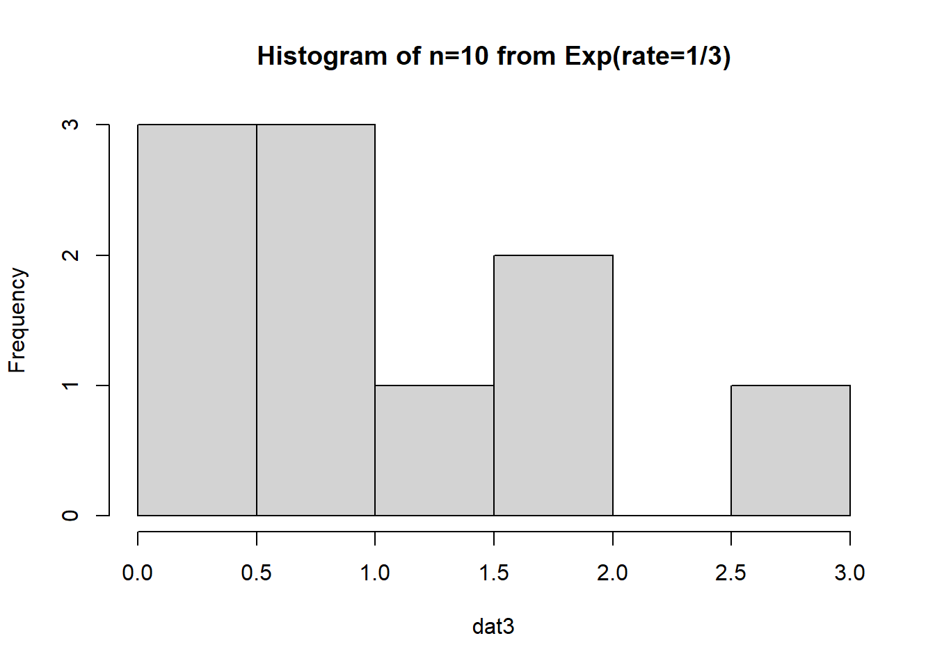
The data appears to be…not normal. Let’s conduct a bootstrap sample with 10,000 bootstrap samples to estimate the sample mean variability:
# note, we set our seed above
n <- length(dat3)
B <- 10000
boot_vec3 <- as.numeric(B)

for(i in 1:B){
  boot_vec3[i] <- mean(sample(dat3, n, replace = TRUE) )
}

hist(boot_vec3, main='Bootstrap Distribution of Sample Mean, n=10 Exponential')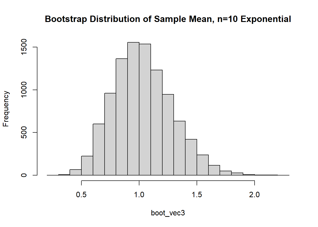
qqnorm(boot_vec3); qqline(boot_vec3)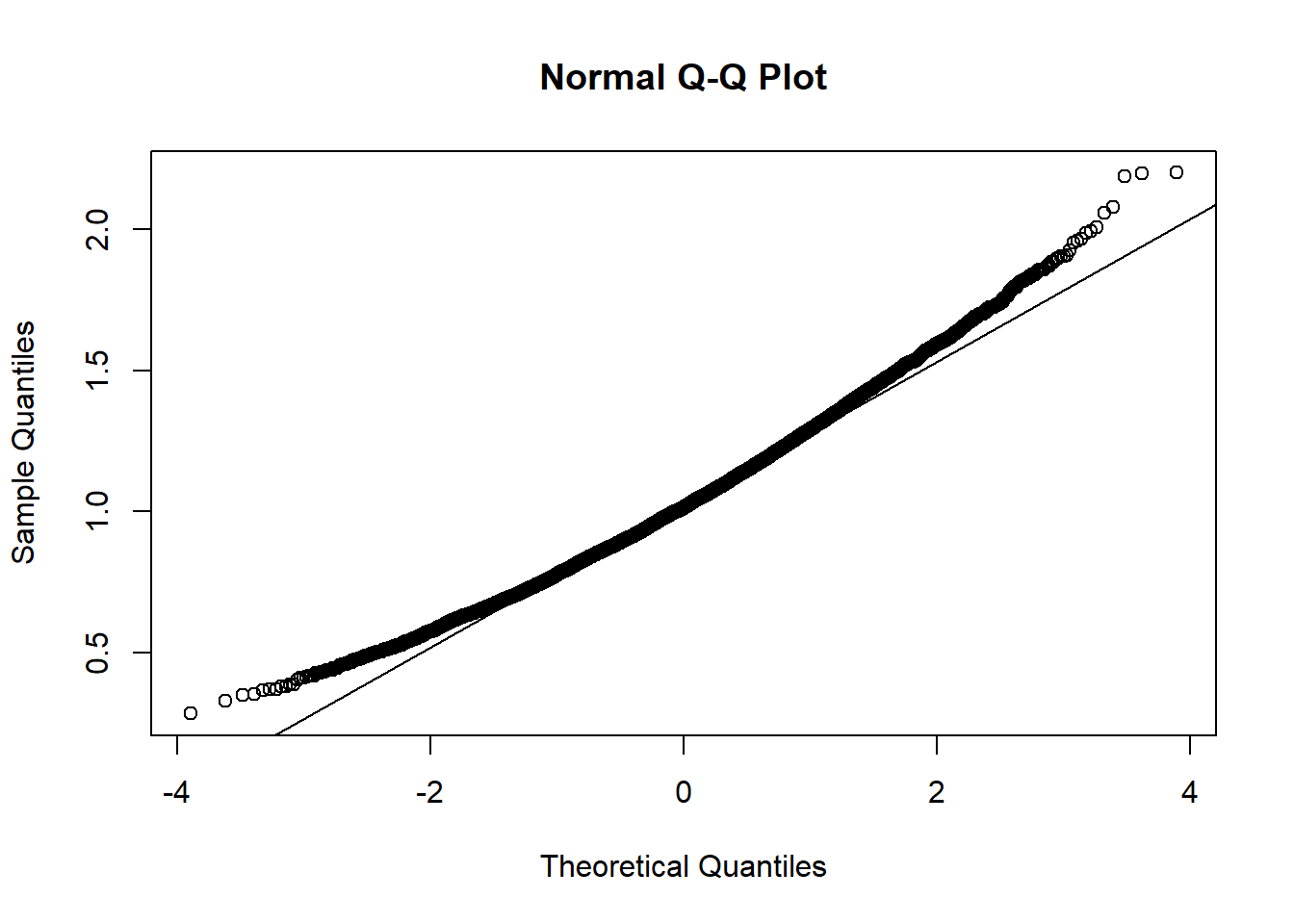
Based on the histogram and QQ plot, the distribution has some right skew (evidence we may need a larger \(n\) for the CLT to really kick in). The 95% normal percentile interval is
#Lower limit of 95% Normal CI
LL <- mean(boot_vec3)-1.96*sd(boot_vec3)
LL
[1] 0.5287681#Upper limit of 95% Normal CI
UL <- mean(boot_vec3)+1.96*sd(boot_vec3)
UL[1] 1.535122sum(boot_vec3 < LL)/B # Coverage of CI at lower end[1] 0.0132sum(boot_vec3 > UL)/B # Coverage of CI at upper end [1] 0.0336We see here the results are NOT close for coverage…we should be concerned about how appropriate the normal percentile CI is. Rather, we can calculate and compare to the bootstrap percentile interval:
quantile(boot_vec3, c(0.025,0.975)) 2.5% 97.5%
0.5814501 1.5796031 Here the two intervals aren’t drastically different, but it isn’t trivial (0.529 vs. 0.581 for LL, 1.535 vs. 1.580 for UL).
For completeness, we can also calculate the ratio of the bias to the standard error to see if it exceeds ±0.10:
# estimate of accuracy for our bootstrap percentile interval
(mean(boot_vec3)-mean(dat3)) / sd(boot_vec3)
[1] -0.01292271What if we have a much larger sample that comes from an exponential distribution?
set.seed(1021)
dat4 <- rexp(n=200, rate=1/3)
hist(dat4, main='Histogram of n=200 from Exp(rate=1/3)')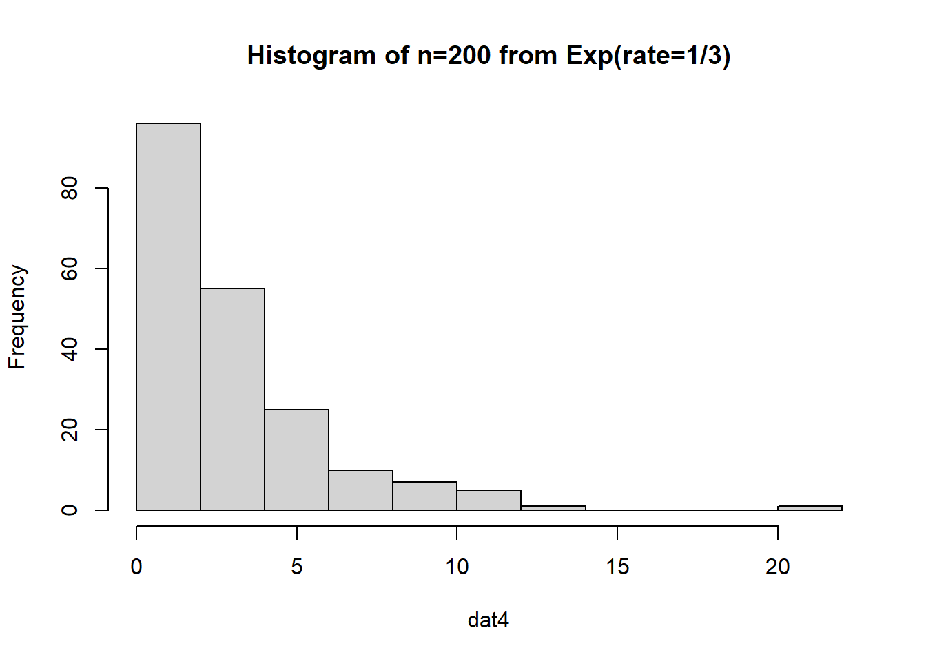
The data is just straight up not normal. To estimate the variability of our sample mean, let’s conduct a bootstrap sample with 10,000 bootstrap samples:
# note, we set our seed above
n <- length(dat4)
B <- 10000
boot_vec4 <- as.numeric(B)

for(i in 1:B){
  boot_vec4[i] <- mean(sample(dat4, n, replace = TRUE) )
}

hist(boot_vec4, main='Bootstrap Distribution of Sample Mean, n=200 Exponential')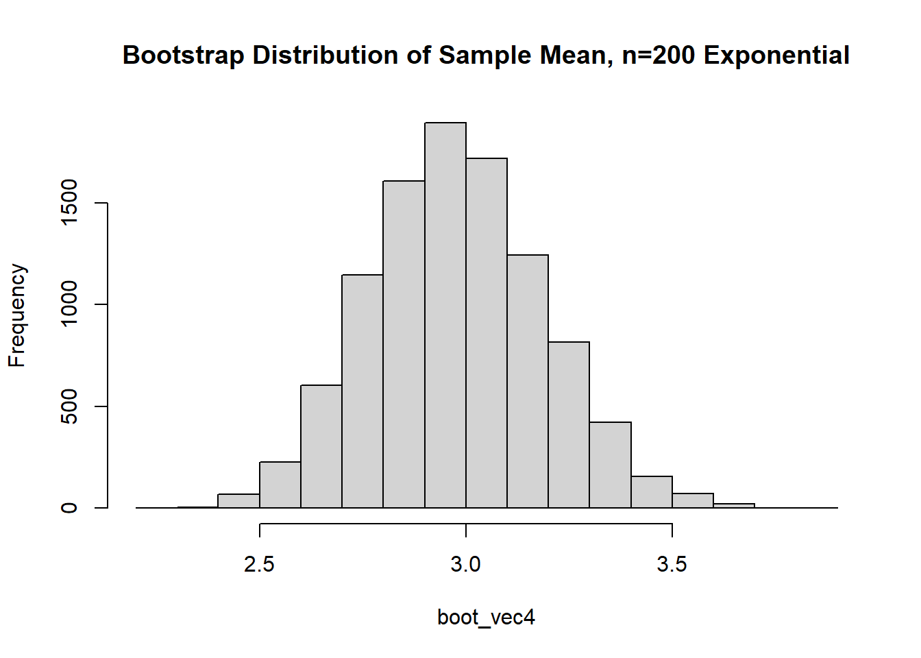
qqnorm(boot_vec4); qqline(boot_vec4)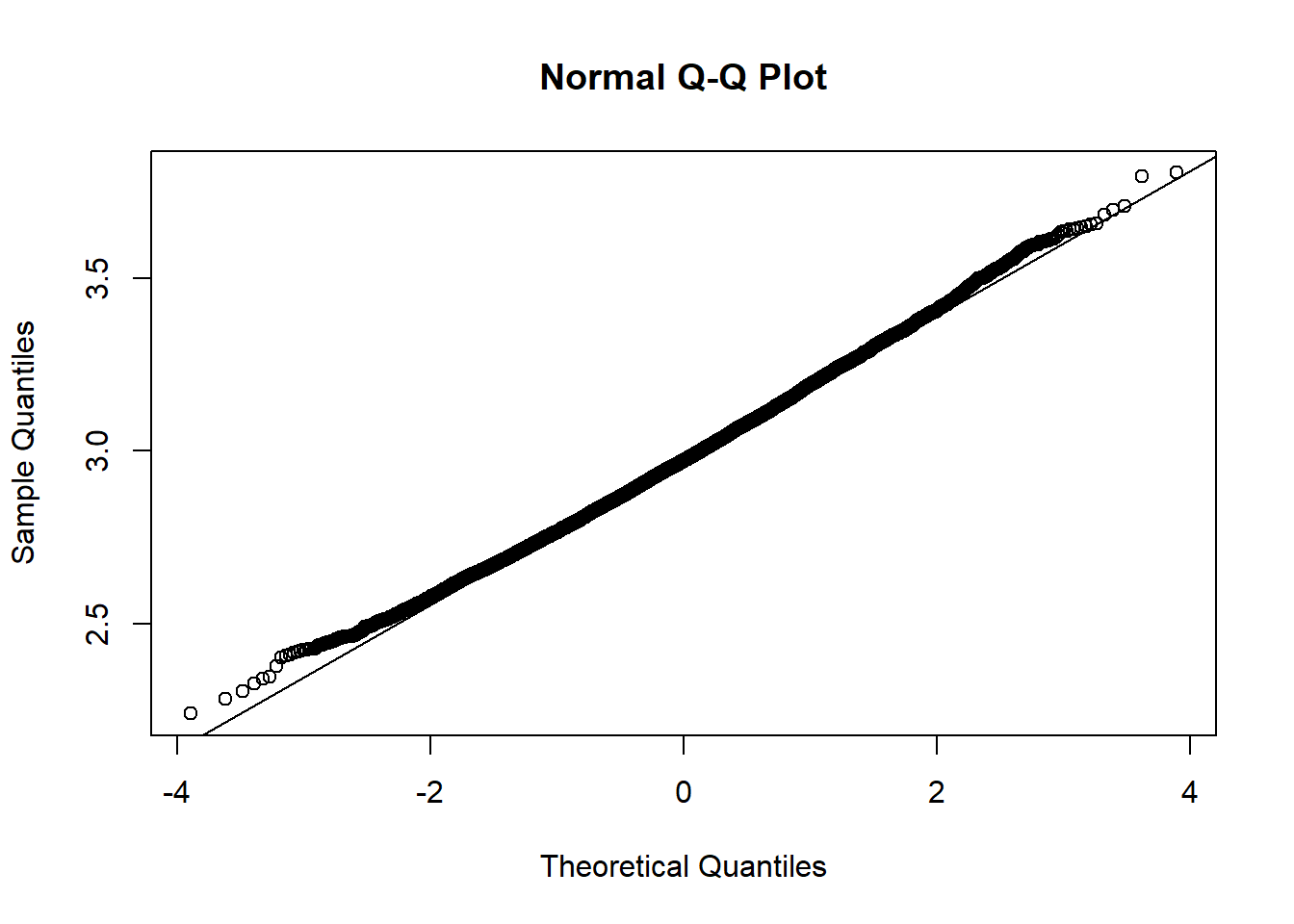
Based on the histogram and QQ plot, the distribution appears decently normal (here the CLT seems to be more applicable given our larger \(n\)). The 95% normal percentile interval is
#Lower limit of 95% Normal CI
LL <- mean(boot_vec4)-1.96*sd(boot_vec4)
LL
[1] 2.566667#Upper limit of 95% Normal CI
UL <- mean(boot_vec4)+1.96*sd(boot_vec4)
UL[1] 3.388219sum(boot_vec4 < LL)/B # Coverage of CI at lower end[1] 0.0207sum(boot_vec4 > UL)/B # Coverage of CI at upper end [1] 0.0283We see here the normal percentile CI is still a bit off from what we would desire, even though the data appears to be generally normal. The bootstrap percentile confidence interval is
quantile(boot_vec4, c(0.025,0.975)) 2.5% 97.5%
2.583263 3.399906 Where we see similar point estimates, but with the percentile intervals we know we are closer to our desired target.
For completeness, we can also calculate the ratio of the bias to the standard error to see if it exceeds ±0.10:
# estimate of accuracy for our bootstrap percentile interval
(mean(boot_vec4)-mean(dat4)) / sd(boot_vec4)
[1] -0.002842806What if we have a much, much larger sample that comes from an exponential distribution?
set.seed(1021)
dat5 <- rexp(n=2000, rate=1/3)
hist(dat5, main='Histogram of n=2000 from Exp(rate=1/3)')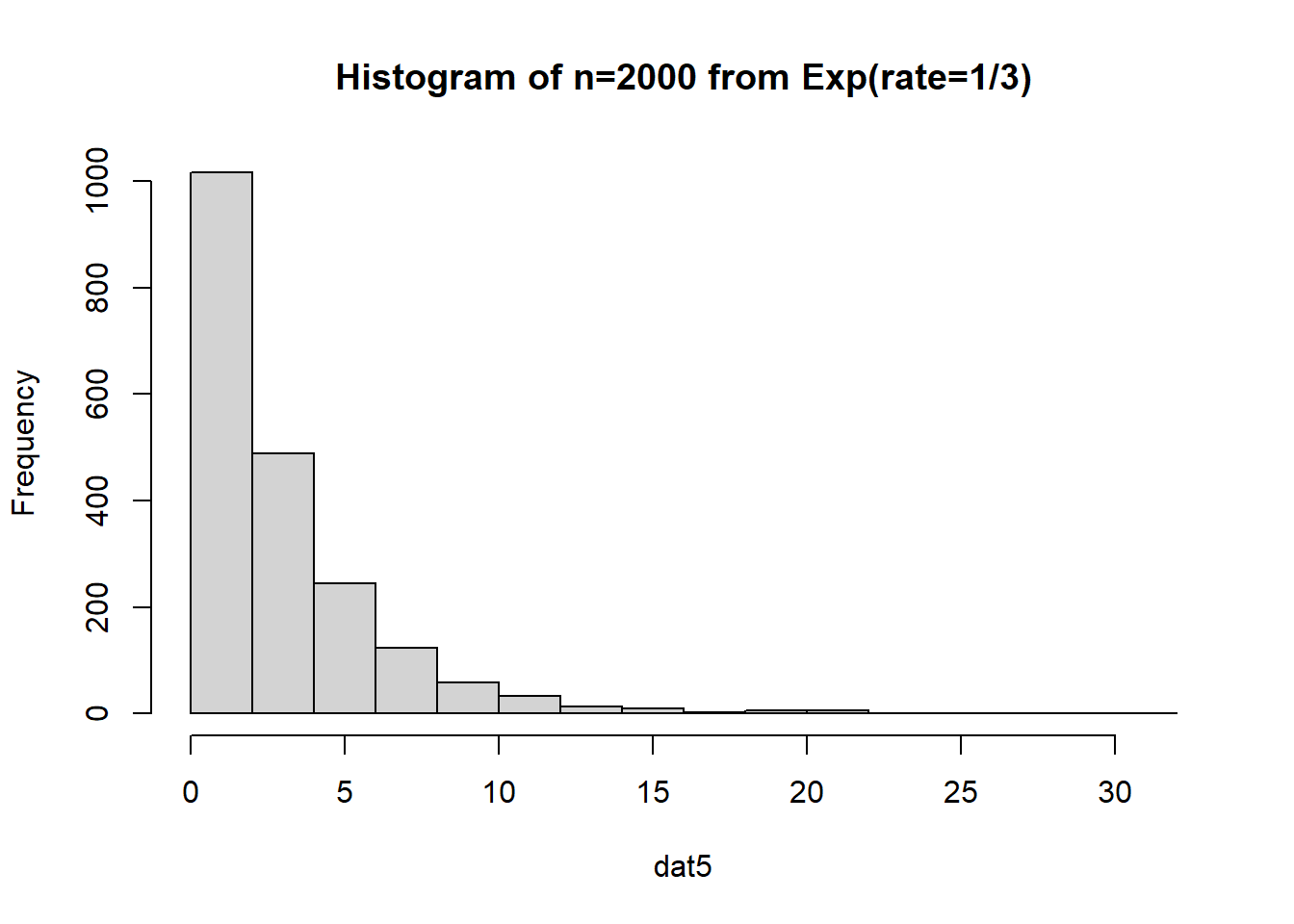
The data is just straight up not normal. To estimate the variability of our sample mean, let’s conduct a bootstrap sample with 10,000 bootstrap samples:
# note, we set our seed above
n <- length(dat5)
B <- 10000
boot_vec5 <- as.numeric(B)

for(i in 1:B){
  boot_vec5[i] <- mean(sample(dat5, n, replace = TRUE) )
}

hist(boot_vec5, main='Bootstrap Distribution of Sample Mean, n=2000 Exponential')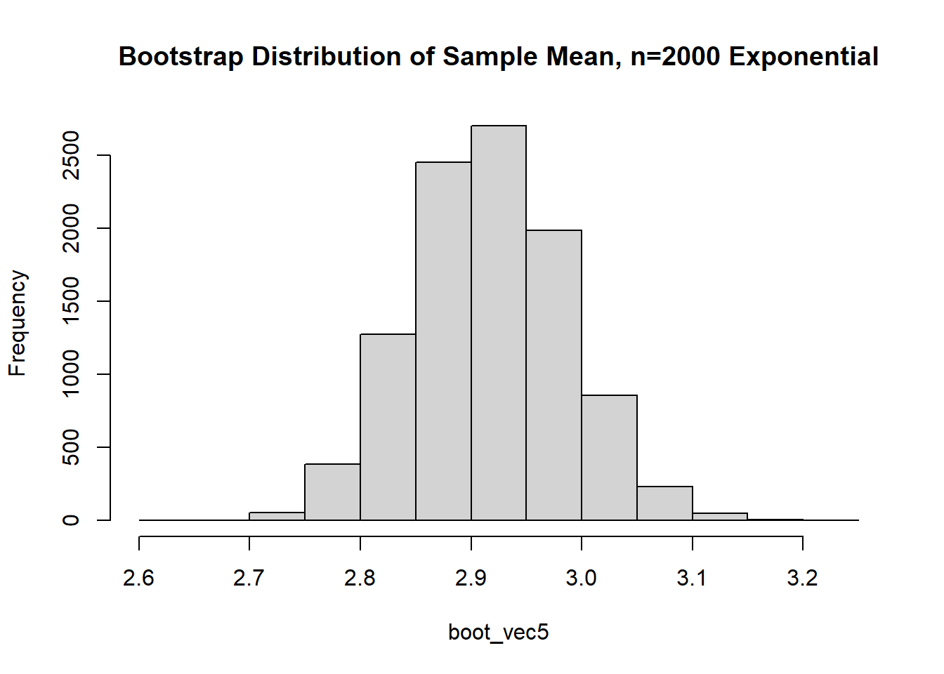
qqnorm(boot_vec5); qqline(boot_vec5)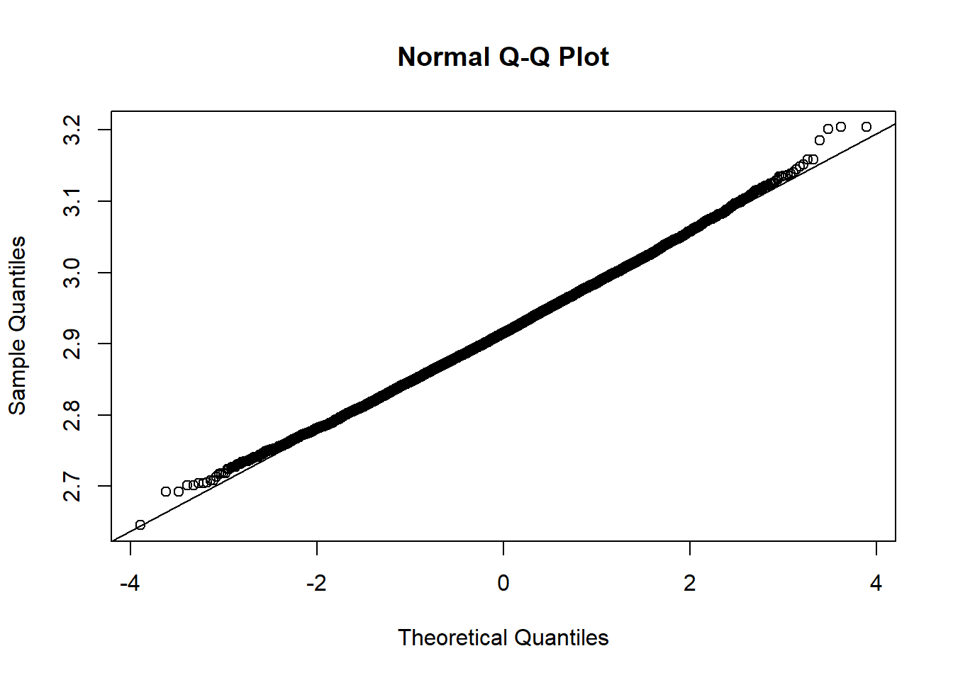
Based on the histogram and QQ plot, the distribution appears decently normal (here the CLT seems to be more applicable given our larger \(n\)). The 95% normal percentile interval is
#Lower limit of 95% Normal CI
LL <- mean(boot_vec5)-1.96*sd(boot_vec5)
LL
[1] 2.779945#Upper limit of 95% Normal CI
UL <- mean(boot_vec5)+1.96*sd(boot_vec5)
UL[1] 3.052643sum(boot_vec5 < LL)/B # Coverage of CI at lower end[1] 0.0218sum(boot_vec5 > UL)/B # Coverage of CI at upper end [1] 0.0265The normal percentile CI is still a bit off from what we would desire, even though the data appears to be even more normally distributed. The bootstrap percentile confidence interval is
quantile(boot_vec5, c(0.025,0.975)) 2.5% 97.5%
2.783262 3.054583 As \(n\) increases, we see that (1) the CLT is more “accurate” (with respect to coverage) and (2) the normal percentile and bootstrap percentile intervals become increasingly similar.
For completeness, we can also calculate the ratio of the bias to the standard error to see if it exceeds ±0.10:
# estimate of accuracy for our bootstrap percentile interval
(mean(boot_vec5)-mean(dat5)) / sd(boot_vec5)
[1] 0.007347859