Simple Linear Regression Assumptions
This page is part of the University of Colorado-Anschutz Medical Campus’ BIOS 6618 Recitation collection. To view other questions, you can view the BIOS 6618 Recitation collection page or use the search bar to look for keywords.
Simple Linear Regression Assumptions
For simple linear regression, our true regression equation is
\[ Y = \beta_0 + \beta_{1} X_{1} + \epsilon, \; \epsilon \sim N(0,\sigma_{e}^2) \]
There are five assumptions we make when using simple linear regression:
Existence: For any fixed value of the variable \(X\), \(Y\) is a random variable with a certain probability distribution having finite mean and variance.
Independence: The errors, \(\epsilon_i\), are independent (i.e., \(Y\)-values are statistically independent of one another).
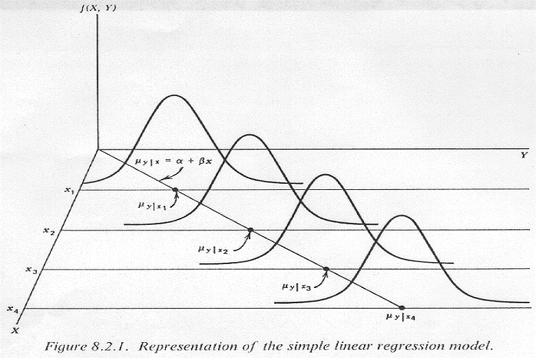
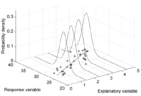
Linearity: The mean value of \(Y\) (or a transformation of \(Y\)), \(\mu_{Y|X}=E(Y)\), is a straight-line function of \(X\) (or a transformation of \(X\)).
Homoscedasticity: The errors, \(\epsilon_i\), at each value of the predictor, \(x_i\), have equal variance (i.e., the variance of \(Y\) is the same for any \(X\)). That is, \[ \sigma_{Y|X}^2 = \sigma_{Y|X=1}^2 = \sigma_{Y|X=2}^2 =... = \sigma_{Y|X=x}^2 \]
Normality: The errors, \(\epsilon_i\), at each value of the predictor, \(x_i\), are normally distributed (i.e., for any fixed value of \(X\), \(Y\) has a normal distribution). (Note this assumption does not state that Y is normally distributed.)
If our data do not meet these assumptions, we have various alternatives to consider (e.g., data transformations, different types of models, etc.). It can be helpful to visualize what the linearity, homoscedasticity, and normality assumptions look like in practice for simple linear regression when we only have one predictor variable. Below are two examples we will walk through:

